
Chi-Square Test in SPSS
Video Walkthrough of a Worked Education Example
This chi-square test in SPSS video asks whether education level is associated with gender among 116 respondents in Crosstabs. The page adds the expected-count check, which test row to quote and why Cramér's V belongs beside the p-value.
WATCH THE VIDEO
Chi-Square Test in SPSS, Start to Finish
Treat the chi-square test of independence as a test of association between two categorical variables, and report its strength beside the p-value. A large p-value is not evidence that the variables are independent. Check the expected counts before the result is read. In this example the Pearson test finds no evidence of an association between gender and education, and Cramér’s V of .098 puts its estimated strength close to zero.
IN SHORT
What the Video Shows in Brief
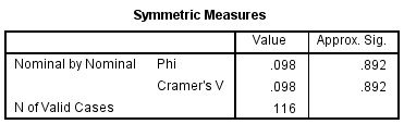
In this chi-square test in SPSS video, 116 respondents are cross-classified by gender (50 male, 66 female) and education (primary school, secondary school, BA, Master, PhD). The path is Analyze, Descriptive Statistics, Crosstabs, with Chi-square and Phi and Cramer’s V ticked under Statistics. The Pearson row gives χ²(4) = 1.111, p = .892, with Cramér’s V = .098 and every expected count at least 7.33: no evidence of an association.
BEFORE YOU RUN
Checks on the Table Before Running Chi-Square
Before you open the SPSS dialogs, the four points below need an answer from your study design and from the data themselves.
One Cell per Case Each respondent falls into exactly one cell, defined by gender and education, and the design settles this. The same people counted twice, or categories measured before and after, call for McNemar's test or a model for related data.
Counts, Not Percentages The test is computed from the observed counts, and the percentages SPSS adds under Cells are for reading the table. Percentages typed in as data, without the counts behind them, cannot be tested.
Expected Counts Large Enough A common guideline asks that no expected count fall below 1 and that no more than 20% fall below 5 (Cochran, 1954). Sparse tables point to Fisher's exact test or to categories merged by a plan made beforehand.
Ordered Categories Carry More Education runs from primary school to PhD, an ordered scale. The Pearson test ignores the order, so a hypothesis about a trend is better served by the linear-by-linear row or an ordinal method, chosen before the output.
STEP BY STEP
Setting Up Crosstabs and Its Statistics Button
The screenshots come from IBM SPSS. Read them alongside the numbered steps below: the menu path, the settings to choose and a check or tip for every step.
Numbered by step, the slides hold the SPSS screen one step at a time. Your release may label a few items differently, since the video was recorded in an older one.
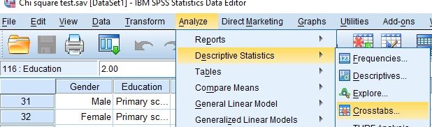
Open the Crosstabs Dialog
Choose Analyze, then Descriptive Statistics, then Crosstabs. The chi-square test of independence is run from Crosstabs, not from the Compare Means submenu.
Check: Two categorical variables belong in this dialog. One categorical variable tested against expected proportions is a goodness-of-fit question and uses a different dialog.
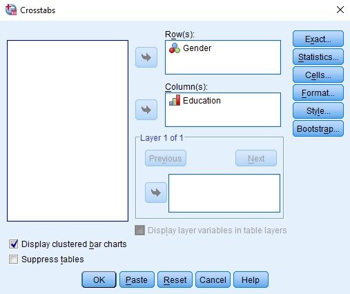
Set the Rows, Columns and Bar Chart
Move Gender into Row(s) and Education into Column(s), then tick Display clustered bar charts. The Exact, Statistics, Cells, Format, Style and Bootstrap buttons are listed at the right edge.
Tip: Swapping rows and columns leaves the test unchanged. It changes which percentages read naturally, so put the group you want to describe in the rows.
Choose the Statistics and Cells
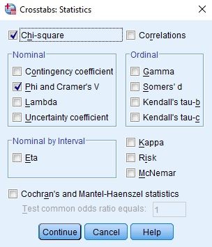
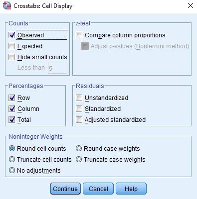
Under Statistics tick Chi-square and Phi and Cramer’s V, then Continue. Under Cells tick Observed counts and the Row, Column and Total percentages, then Continue and OK.
Watch: The chi-square statistic says nothing about strength, which is why Phi and Cramer’s V are ticked. Tick Expected counts as well when the table is small, to read them cell by cell.
Confirm 116 Valid Cases in the Summary
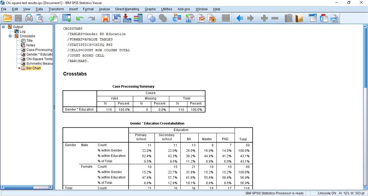
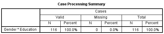
The Viewer shows the CROSSTABS syntax, then the Case Processing Summary with valid, missing and total cases. Confirm that the valid N matches the number of respondents you expect.
Check: A respondent with gender or education missing is left out of the table, and SPSS gives no warning. If the valid N falls short of the respondents surveyed, find the gap before reading the test.
Read the Crosstabulation
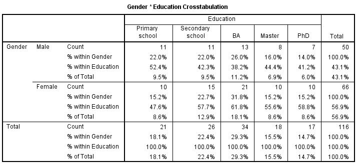
The Gender by Education table lists the count and three percentages in each cell: within Gender, within Education and of Total. Read the counts first, then the percentage that matches your question.
Watch: Percent within Gender answers how educated men and women are, and percent within Education answers who makes up each level. The two are easy to mix up, so name the direction.
Read the Test and the Effect Size
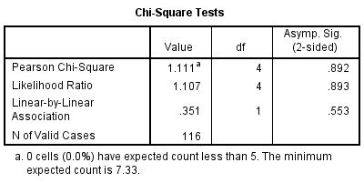
The Chi-Square Tests table gives the Pearson row, the Likelihood Ratio, the Linear-by-Linear Association and a footnote on expected counts. Symmetric Measures then gives Phi and Cramer’s V with their approximate significance.
Tip: Read the footnote before the Pearson row. In a table with two rows, Phi and Cramer’s V take the same value, and the p-value beside them repeats the Pearson result.
Look at the Clustered Bar Chart
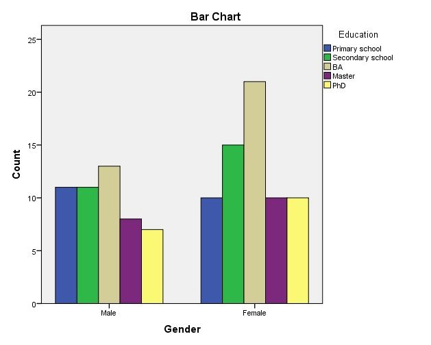
The last output item is a bar chart of counts, with Gender on the horizontal axis and one bar per education level. It shows the shape of the table at a glance but does not test it.
Check: The bar colors follow Education in the order of its codes, from primary school to PhD, so match the legend to the table before describing any bar.
READING THE OUTPUT
Reading the Crosstabulation and Chi-Square Tests
Each row of the table names one value in the SPSS output, gives its figure in the video example and says how to read it for your own data.
| Output value | In the example | How to read it |
|---|---|---|
| Valid N | 116 (100.0%), 0 missing | Cases with both variables. Degrees of freedom are (rows minus 1) times (columns minus 1), which gives 4 here |
| Counts by Gender | Male 50, Female 66 | Row totals. Education totals are 21, 26, 34, 18 and 17 |
| % within Gender | Male 22.0, 22.0, 26.0, 16.0, 14.0; Female 15.2, 22.7, 31.8, 15.2, 15.2 | Each row sums to 100%. Compare the two rows level by level |
| Pearson Chi-Square | 1.111, df 4, Asymp. Sig. .892 | The row to report for this table. Asymp. Sig. is a large-sample approximation, which the expected counts support here |
| Likelihood Ratio | 1.107, df 4, .893 | An alternative test statistic that agrees closely with Pearson here |
| Linear-by-Linear Association | .351, df 1, .553 | A test for a linear trend across ordered categories. It is meaningful only if the order is real |
| Expected count footnote | 0 cells (0.0%) below 5, minimum 7.33 | The check on the table. Every expected count is above 5 here |
| Phi and Cramer’s V | .098 and .098, Approx. Sig. .892 | The strength of the association, on a scale from 0 to 1. Both are close to zero |
COMMON MISTAKES
Slips With Cell Weights, the Null and Cramér's V
Here are six mistakes made with this chi-square test in the data, the dialogs, the output or the write-up, each with a short way to avoid it.
A Null Hypothesis Stated as Dependence The null hypothesis is that the two variables are independent, and the alternative is that they are associated. Writing them the other way round turns every conclusion upside down.
A Large p Read as Proof of No Link A p-value of .892 shows no evidence of an association. It does not show that gender and education are unrelated, and a table with few cases could hide a real association.
Cramér's V Confused With the p-Value Cramér's V here is .098, and .892 is the p-value printed in the same row of the table. Mixing them up reports a strong association where the data show almost none.
Cell Counts Entered Without Weighting A table typed in as one row per cell with a count column needs Data, Weight Cases set to that column. Without it, Crosstabs counts each of the 10 rows once, and N becomes 10 instead of 116.
Gender Share Mixed With Education Share Of the 21 respondents in the primary school category, 47.6% are female, while 15.2% of women fall in that category. The two percentages differ, so name the one quoted.
Bar Heights Compared Across Unequal Groups The chart shows counts, and the table has 50 men and 66 women. Taller female bars reflect the larger group, so read the pattern within each gender or use the row percentages.
If you have already run this test, Independent Statistical Review has an OnlineSPSS statistician check the expected counts, the row and V against your output.
SOURCES
Sources and Further Reading
The sources below support statements made on this page, and the line under each entry says what to read it for.
Cochran, W. G. (1954). Some methods for strengthening the common χ2 tests. Biometrics, 10(4), 417-451. DOI: 10.2307/3001616
Read this for the origin of the expected-count guideline for chi-square tests.
Cohen, J. (1988). Statistical power analysis for the behavioral sciences (2nd ed.). Lawrence Erlbaum Associates.
Read this for the benchmarks for w and how w relates to Cramér's V.
FREQUENTLY ASKED QUESTIONS
Menus, Expected Counts and Strength in the Example
Four questions on this chi-square test are answered here: an SPSS screen that differs from the video, the method, the example figures and the write-up.
Why does the Crosstabs dialog look different in my SPSS?
The video was recorded in an older release of IBM SPSS Statistics. Crosstabs is still reached through Analyze, then Descriptive Statistics, although the Compare Means submenu is renamed in recent releases. The Row(s) and Column(s) boxes, the Statistics and Cells buttons and the bar chart tick match the video.
Why does the footnote on expected counts matter?
The Pearson test relies on a large-sample approximation that is poor when expected counts are small. In this table 0 cells have an expected count below 5 and the smallest is 7.33, so the guideline (Cochran, 1954) is met and the Pearson row can be read. Otherwise, the Exact button offers exact p-values where the Exact Tests option is licensed.
How strong is the association in the example?
Cramér’s V is .098, and Phi is the same because the table has two rows. For such a table V equals Cohen’s w, whose conventional benchmarks are .10, .30 and .50 (Cohen, 1988), so .098 sits just below small. The benchmarks are conventions, and the field decides what counts as meaningful.
Which figures from the 2 by 5 education table go into a write-up?
With the test, df, sample size, p-value and a named measure of association, in words that say association and not cause. No evidence of an association between gender and education was found, χ²(4, N = 116) = 1.11, p = .892, Cramér’s V = .098, with no expected count below 7.33.
NEXT STEP
Need a Contingency Table
Analyzed or Checked?
OnlineSPSS is a statistical consultancy for researchers. Share your design and dataset, and a statistically trained Research Coordinator reviews it. The scope and one fixed project fee are confirmed before work begins.
No Commitment Required
Strictly Confidential
Fixed Project Fee
In-House PhD-Level Statisticians
Same-Day Response
Serving Researchers Since 2014