
Simple Linear Regression in SPSS
Video Walkthrough of a Worked Slope Example
This simple linear regression in SPSS video predicts a happiness rating from a depression score for 59 cases in the Linear Regression dialog. The page adds what the slope and R squared say, which conditions concern the residuals and how F relates to t.
WATCH THE VIDEO
Simple Linear Regression in SPSS, Start to Finish
Report the slope in the units of the outcome with its 95% interval, and give R squared beside it. The p-value alone says only how unusual a slope this steep would be if the population slope were zero. Here B = -.128 happiness points per depression point, 95% CI [-.240, -.017], with R squared = .085, so depression accounts for a small share of the variation in happiness across 59 cases.
IN SHORT
What the Video Shows in Brief
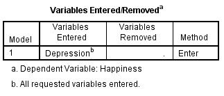
In this simple linear regression in SPSS video, Happiness (1 to 5) is the dependent variable and Depression (1 to 10) the only independent variable for 59 cases, with the Enter method. The path is Analyze, Regression, Linear. The slope is B = -.128, 95% CI [-.240, -.017], p = .025, and R squared is .085: statistically significant, and the interval excludes zero.
BEFORE YOU RUN
Scale, Line and Residuals Before Linear Regression
Four points about your design and your data come first. Each of them is decided before this simple regression is run in SPSS.
A Quantitative Outcome Happiness is one rating from 1 to 5, with 17 of 59 cases at 5 and four at 1. The line treats the five steps as equal, which is an approximation for a rating, and ordinal regression is the alternative that does not.
A Straight-Line Pattern The model fits one straight line to the average happiness at each depression score. A curve would leave a pattern in the residuals, so a scatterplot of the two variables is the first look, and the video requests only the residual plot.
Conditions on the Residuals Constant spread and, in smaller samples, roughly normal errors concern the residuals, not Happiness or Depression themselves (Ernst & Albers, 2017). Larger samples relax the normality condition for the slope (Lumley et al., 2002).
Independent Cases Each of the 59 cases is a separate person with one pair of scores. Pairs that share a class or a clinic make the residuals dependent, and then the interval for B is usually too narrow.
STEP BY STEP
Setting Up Linear Regression With a Single Predictor
Menu path, settings and a check or tip: the numbered steps below give all three for every step of this simple regression, with screenshots from IBM SPSS.
Numbered by step, the slides hold the SPSS screen one step at a time. Your release may label a few items differently, since the video was recorded in an older one.

Open the Linear Regression Dialog
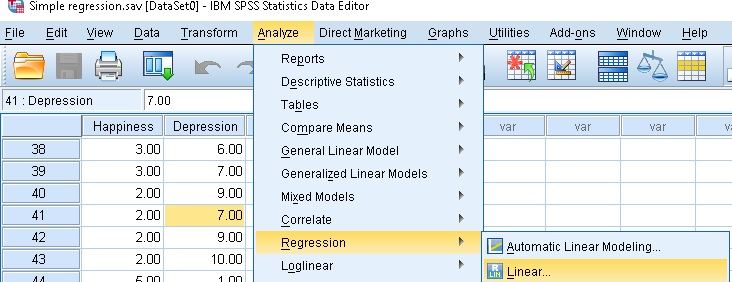
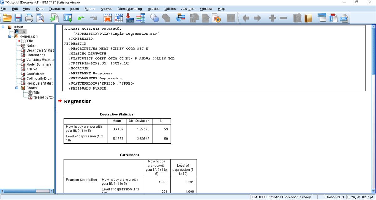
Choose Analyze, then Regression, then Linear. The grid beneath the menu lists Happiness and Depression side by side, a case in each row, and the submenu shows Automatic Linear Modeling above Linear.
Check: Linear is the entry for one quantitative outcome and predictors chosen by you. Automatic Linear Modeling, listed just above it, prepares the data and selects predictors on its own, which one prespecified predictor does not need.
Place Happiness and Depression in Their Boxes
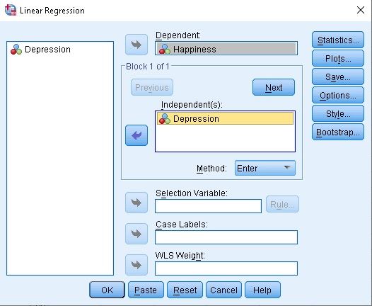
Move Happiness into the Dependent box and Depression into the Independent(s) box, and leave Method on Enter. Statistics, Plots, Save, Options, Style and Bootstrap are the buttons on the right.
Watch: The two roles are not interchangeable. Swapping the boxes gives a different slope and interval, while R squared stays the same, so the research question decides which variable is the outcome.
Tick the Options in the Statistics Dialog
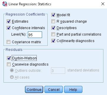
Select Statistics. Estimates, Confidence intervals (Level 95), Model fit, Descriptives and Collinearity diagnostics are ticked, as is Durbin-Watson under Residuals. Select Continue.
Tip: Collinearity diagnostics compare predictors with one another, and one predictor has no partner. The tick adds nothing in a model like this one, and the extra table is easy to mistake for a check that was needed.
Pick *ZRESID and *ZPRED in the Plots Dialog
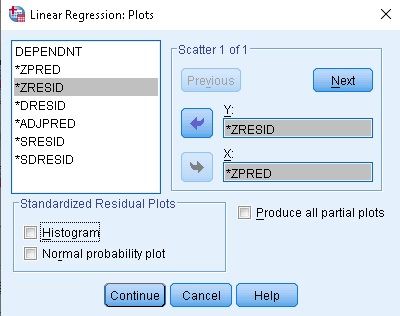
Select Plots, move *ZRESID into Y and *ZPRED into X, and leave Histogram and Normal probability plot unticked. Select Continue, then OK. This requests one scatterplot of standardized residuals against standardized predicted values.
Check: The screenshots show this dialog but no chart. The Viewer outline lists a *zresid chart, and that is where curvature and unequal spread are judged, which the F test and the interval rely on.
Check the Log, Descriptives and Correlations
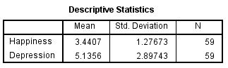
The Viewer starts with the REGRESSION syntax, whose lines include /MISSING LISTWISE and /METHOD=ENTER Depression. Descriptive Statistics gives N = 59 for both variables, and Correlations and Variables Entered/Removed follow.
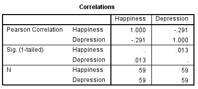
Watch: The correlation table prints Sig. (1-tailed) for r = -.291, so its .013 is half the two-tailed p of .025 that the Coefficients table shows for the slope. Quote the two-tailed value.
Read the Model Summary and ANOVA Tables
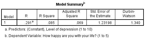
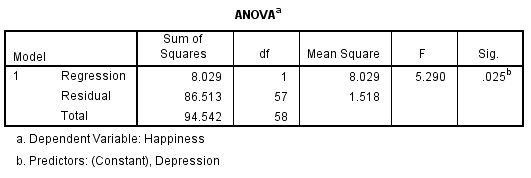
Model Summary prints R .291, R Square .085, Adjusted R Square .069, a standard error of the estimate of 1.23198 and Durbin-Watson 1.340. ANOVA gives F(1, 57) = 5.290, p = .025 for the model.
Check: R is printed as .291 although r is -.291, because R is the correlation between observed and predicted happiness and cannot be negative. The sign of the slope is read in the Coefficients table.
Read the Coefficients Table
The Depression row gives B -.128, Std. Error .056, Beta -.291, t -2.300, Sig. .025 and a 95% interval for B of -.240 to -.017. (Constant) is 4.100, the fitted happiness at a depression score of 0, which lies below the 1 to 10 scale.
Tip: With one predictor, Beta equals r (-.291) and t squared equals the ANOVA F, since 2.300 squared is 5.29. The table and the ANOVA are two views of one test, so their p-values cannot disagree.
READING THE OUTPUT
Reading the Model Summary, ANOVA and Coefficients
Each value below comes from the SPSS output. Its row shows the figure in the video example, then how to interpret it when the data are your own.
| Output value | In the example | How to read it |
|---|---|---|
| Mean and Std. Deviation | Happiness 3.4407 and 1.27673, Depression 5.1356 and 2.89743 | Means and spread of each variable for the 59 cases the model uses. Report them with the model |
| Pearson Correlation and Sig. (1-tailed) | -.291 and .013 | The correlation of outcome and predictor, printed with a one-sided p as the Sig. label says |
| R, R Square and Adjusted R Square | .291, .085 and .069 | The share of variance in happiness that the line accounts for in this sample, with a version corrected for the number of predictors |
| Std. Error of the Estimate | 1.23198 | The typical distance of an observed rating from the fitted line, in rating points |
| Durbin-Watson | 1.340 | A statistic for correlation between neighboring residuals in file order, where 2 marks none |
| F and Sig. in ANOVA | 5.290 and .025, df 1 and 57 | Tests the fitted line against a flat line at the mean of happiness. Regression and Residual rows hold the sums of squares |
| B and 95% Confidence Interval | -.128, -.240 to -.017 | The difference in average happiness per depression point, and the slopes compatible with the data |
| Std. Error and Sig. of B | .056 and .025 | Uncertainty of the slope and the two-sided p for a population slope of zero. The p-value does not measure size |
COMMON MISTAKES
Slips With Dropped Cases, R Squared and Slope Wording
Six mistakes follow, each tied to a stage (data setup, SPSS dialogs, output or write-up) and each paired with a brief note on how to avoid it.
Cases Dropped Without a Message The Log shows /MISSING LISTWISE, so a case missing either Happiness or Depression leaves the model silently. Compare N = 59 in Descriptive Statistics with the rows in the Data Editor before reading anything else.
The ANOVA Label Read as a Group Test The ANOVA table here is the F test of the regression, with 1 and 57 df, not a comparison of group means. Quoting it as a one-way ANOVA confuses readers, so call it the F test of the model.
R Squared Judged on Its Own An R squared of .085 does not make the slope worthless, and a high one would not make it right. Read it with the slope and its interval, and against the usual values for such ratings, before calling the fit weak.
A Durbin-Watson Value Read Alone The 1.340 describes neighboring residuals in file order. A value below 2 points to positive correlation between neighbors, which matters only if the order means something, such as time or class, so check how the rows were entered.
Fitted Values Read as Ratings The line gives about 3.97 at Depression 1 and 2.82 at 10 (computed outside SPSS). These are average happiness at that score, not ratings any case could give, and single ratings scatter around them by about 1.23 points.
A Slope Worded as a Cause Cases one depression point higher score .128 lower on average. Wording such as raising depression lowers happiness describes a change within a person, which a single set of 59 cases cannot show.
If you have already run this test, Independent Statistical Review has an OnlineSPSS statistician check the slope, the interval and the wording against your output.
SOURCES
Sources and Further Reading
A note under each reference says what to read it for, and every reference listed supports a statement on this page.
Ernst, A. F., & Albers, C. J. (2017). Regression assumptions in clinical psychology research practice: A systematic review of common misconceptions. PeerJ, 5, Article e3323. DOI: 10.7717/peerj.3323
Read this for why the normality condition concerns errors, not variables.
Lumley, T., Diehr, P., Emerson, S., & Chen, L. (2002). The importance of the normality assumption in large public health data sets. Annual Review of Public Health, 23(1), 151-169. DOI: 10.1146/annurev.publhealth.23.100901.140546
Read this for how large samples relax the normality condition.
FREQUENTLY ASKED QUESTIONS
Menus, Slope Intervals and Ordinal Models in the Example
Four questions are answered here. They deal with the SPSS screens, the method behind this analysis, the example in the video and how to report what it shows.
Why does the Linear Regression dialog look different in my SPSS?
The video was recorded in an older release of IBM SPSS Statistics. The Statistics page in IBM’s release 30 documentation still lists Estimates, Confidence intervals, Model fit, Descriptives and Collinearity diagnostics. Its Residuals entry offers Durbin-Watson beside a PRESS statistic, which the video’s Statistics dialog does not show.
What does the interval for B, -.240 to -.017, say about the slope?
It holds the slopes compatible with the data at the 95% level. Across the observed depression range of 1 to 10, nine steps, the fitted happiness would differ by about 0.15 to 2.2 points (computed outside SPSS), so the data fit anything from a very flat to a clearly falling line.
Would ordinal regression suit the 1-to-5 happiness rating better?
Linear regression treats the five steps as equal, while ordinal regression models the odds of a higher category and does not. With one predictor either can be run, and the choice belongs in the analysis plan. The ratings here fall in all five categories (4, 11, 16, 11 and 17 cases), which alone is no reason to switch.
How are B = -.128, R squared = .085 and F(1, 57) = 5.29 written up?
Report the slope, its interval, the fit and the test. Depression predicted happiness in 59 cases, B = -.128, 95% CI [-.240, -.017], t(57) = -2.30, p = .025, R squared = .085 (adjusted .069), F(1, 57) = 5.29. Means and SDs, 3.44 and 1.28 for happiness and 5.14 and 2.90 for depression, belong in the same paragraph.
NEXT STEP
Need a One-Predictor Model
Run or Checked?
OnlineSPSS is a statistical consultancy for researchers. Share your design and dataset, and a statistically trained Research Coordinator reviews it. The scope and one fixed project fee are confirmed before work begins.
No Commitment Required
Strictly Confidential
Fixed Project Fee
In-House PhD-Level Statisticians
Same-Day Response
Serving Researchers Since 2014