
Paired Samples t-Test in SPSS
Video Walkthrough of a Worked Pre-Post Example
This paired samples t-test in SPSS video compares the math test scores of 37 cases at two time points in the Paired-Samples dialog. The page adds what the pairs need, why the sign of the difference matters and what its 95% confidence interval allows.
WATCH THE VIDEO
Paired Samples t-Test in SPSS, Start to Finish
Judge the paired test on the differences, not on the two columns: the mean change with its 95% interval is the result, and the correlation table only describes the pairing. Name the direction of subtraction, and call a change between two occasions a change, not the effect of the training. In this example the scores fell by 4.24 points on average and the interval includes zero.
IN SHORT
What the Video Shows in Brief
In this paired samples t-test in SPSS video, the math test results of 37 cases at time 1 and time 2, before and after a training session, are compared. The path is Analyze, Compare Means, Paired-Samples T Test, with the two scores entered as Pair 1. Time 1 averages 73.08 and time 2 averages 68.84, so the mean difference (Time 1 minus Time 2) is 4.24 points, 95% CI [-3.68, 12.16], t(36) = 1.09, p = .284: not statistically significant, and the interval includes zero.
BEFORE YOU RUN
Checks on Pairs and Difference Scores Before Pair 1
Here are four points to settle about your study design and your data, each one ahead of running this paired t-test in SPSS.
Genuine Pairs Each row holds two measurements from one case, or from two matched cases, and the design settles that. Two separate groups call for the independent test, and three or more occasions for a repeated measures model.
One Outcome on One Scale Both columns measure the same outcome in the same units, so that their difference means something. An ordinal outcome points to the Wilcoxon signed-rank test when differences can be ranked by size, or to the sign test when they cannot.
Shape of the Differences The test concerns the mean of the differences, so inspect their histogram, not the two columns. With 37 pairs, a test of the mean difference copes with moderate skew (Lumley et al., 2002), but a few extreme differences can move it.
A Design That Supports the Question Two occasions with no comparison group cannot separate the training from practice, other events or regression toward the mean. Without such a group, the result describes a change over time.
STEP BY STEP
Filling the Paired Variables Grid in the Dialog
Screens are pictured as they appear in IBM SPSS, and each numbered step below sets out the menu path, the settings to select and one check or tip.
Each numbered slide captures what SPSS displays at one step of this paired t-test. The recording comes from an older release, so a few labels may not match your version.

Open the Paired-Samples Dialog
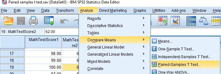
Choose Analyze, then Compare Means (Compare Means and Proportions in recent releases), then Paired-Samples T Test.
Check: Pairs of scores, from one group measured twice or from matched cases, belong in this dialog. Unrelated groups, or one mean set against a fixed value, belong in the Independent-Samples and One-Sample T Test dialogs.
Start From the Empty Pair
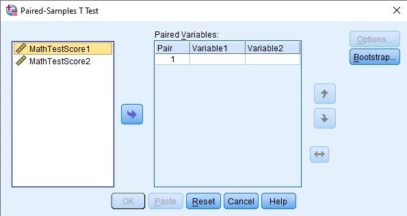
The dialog opens with the variables listed on the left (MathTestScore1 and MathTestScore2) and an empty Pair 1 row in the Paired Variables grid. OK and Paste stay grayed out until a complete pair is entered.
Tip: Click the first variable in the list to enable the arrow button. A second pair can be added on the next grid row, and every pair gets its own test.
Enter the Two Scores as Pair 1
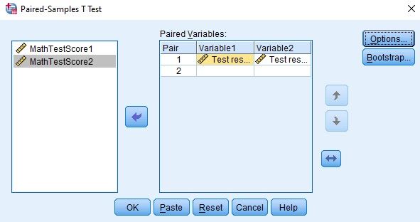
Move MathTestScore1 into Variable1 and MathTestScore2 into Variable2 of Pair 1, then select OK. The confidence level sits under Options and stays at 95% unless changed.
Watch: The difference is Variable1 minus Variable2, here Time 1 minus Time 2, so a positive mean means the scores fell. Enter the earlier occasion first only if that is the order you will name in the write-up.
Confirm the Pair in the Viewer Log
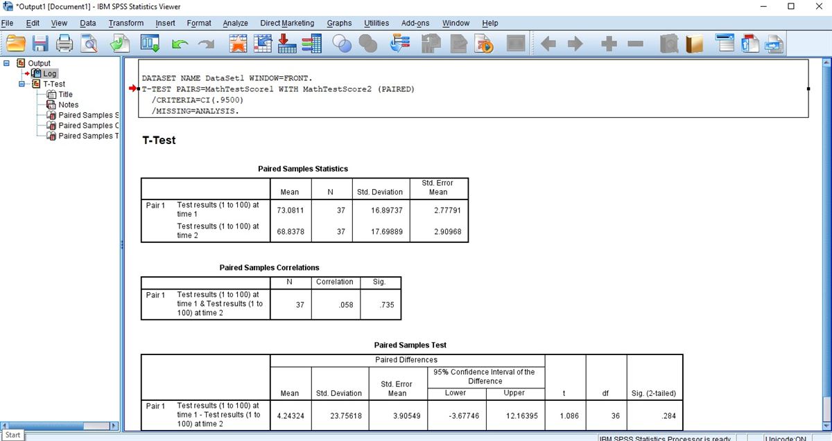
The Viewer shows the command T-TEST PAIRS=MathTestScore1 WITH MathTestScore2 (PAIRED) with CRITERIA=CI(.9500) and MISSING=ANALYSIS, followed by the three tables. Confirm that the pair in the command is the pair you meant.
Check: A case with one of the two scores missing is dropped from the test without a message. The N in the first table is the clearest trace of it, so check it against the cases in the file.
Read the Paired Samples Statistics
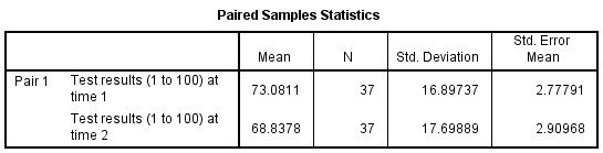
The first table gives the Mean, N, Std. Deviation and Std. Error Mean for each occasion. These describe the two columns, and the test itself is in the third table.
Check: Means and SDs appear to four or five decimals here. Rounding them, not cutting them short, turns 68.8378 into 68.84 and an SD of 17.69889 into 17.70, not 68.83 and 17.69.
Read the Paired Samples Correlations
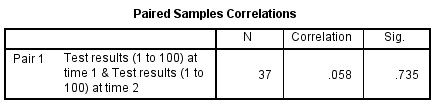
The second table gives the correlation between the two scores across the pairs, with its N and Sig. It describes how the pairing behaves and does not test the change.
Watch: Two tests of the same people are usually related, so a correlation near zero is a prompt to check that each row really holds one person’s two scores.
Read the Paired Samples Test
The third table gives the mean, SD and standard error of the differences, the 95% confidence interval of the difference, t, df and Sig. (2-tailed). Interpret the interval and the mean difference together, not the p-value alone.
Tip: Recent releases split the p column into One-Sided p and Two-Sided p. Quote the two-sided value unless a one-sided test was planned before the data were seen.
READING THE OUTPUT
Reading Paired Samples Statistics, Correlations and Test
Row by row, the table names a value in the SPSS output for this paired t-test, its figure in the video example and how to read it in your data.
| Output value | In the example | How to read it |
|---|---|---|
| N | 37 | Complete pairs only, since a case missing either score is left out. The test has N minus 1 degrees of freedom, here 36 |
| Mean | Time 1 73.0811, Time 2 68.8378 | The mean of each occasion, reported as 73.08 and 68.84 |
| Std. Deviation | 16.89737 and 17.69889 | The spread of each occasion, reported as 16.90 and 17.70. It is not the spread of the differences |
| Correlation and Sig. | .058 and .735 | How closely the two scores move together across cases. It describes the pairing, not the change |
| Paired Differences Mean | 4.24324 | Time 1 minus Time 2, because Time 1 was entered first. A positive value means the scores fell on average |
| Std. Deviation and Std. Error Mean | 23.75618 and 3.90549 | The spread of the 37 differences, and the SD of those differences over the square root of N |
| 95% CI of the Difference | -3.67746 to 12.16395 | The mean changes consistent with the data. It spans zero, so neither a rise nor a fall is ruled out |
| t, df and Sig. (2-tailed) | 1.086, 36 and .284 | The mean change divided by its standard error, with two-sided p. Neither figure is a measure of the size of the change |
COMMON MISTAKES
Slips With Variable Order, Correlation df and Pairing
Here are six mistakes made with this paired t-test in the data, the dialogs, the output or the write-up, each with a short way to avoid it.
A Low Correlation Left Unexamined A correlation of .058 between two scores of the same people is unusually low. It can be genuine, or it can mean the rows are not aligned, so check the pairing before trusting the test.
The Later Occasion Entered First SPSS subtracts Variable2 from Variable1. Entering time 2 first reverses the sign of the mean difference and of t, and an unchanged sentence about improvement would then say the opposite.
Reading p = .284 as No Effect of Training A p above .05 leaves a real change unconfirmed, not disproved. The interval, 3.68 points below to 12.16 above zero, shows which changes remain compatible, and the design cannot isolate a training effect.
Degrees of Freedom for the Correlation The correlation uses N minus 2 degrees of freedom, here 35, while the test uses N minus 1, here 36. Writing r(37) takes the sample size for the df.
Differences Never Plotted The Paired-Samples dialog has no plot option, and the video shows no plot. A new variable holding time 1 minus time 2 gives a histogram of the quantity the test is about.
Paired Scores Run as Independent Groups Stacking both scores in one column with a time code and running the Independent-Samples T Test treats 37 people as 74 cases. The pairing is lost, and so are the right standard error and df.
If you have already run this test, Independent Statistical Review has an OnlineSPSS statistician check the pairing, the sign and the interval against your output.
SOURCES
Sources and Further Reading
The reading below supports what this page says about this paired t-test, and a line under each entry notes what to read it for.
Lumley, T., Diehr, P., Emerson, S., & Chen, L. (2002). The importance of the normality assumption in large public health data sets. Annual Review of Public Health, 23(1), 151-169. DOI: 10.1146/annurev.publhealth.23.100901.140546
Read this for when a t-test of a mean holds up with skewed data.
Lakens, D. (2013). Calculating and reporting effect sizes to facilitate cumulative science: A practical primer for t-tests and ANOVAs. Frontiers in Psychology, 4, Article 863. DOI: 10.3389/fpsyg.2013.00863
Read this for how dz and dav are built for paired data.
FREQUENTLY ASKED QUESTIONS
Menus, Difference Scores and Effect Size in the Example
Four questions on this paired t-test are answered here: an SPSS screen that differs from the video, the method, the example figures and the write-up.
Why does the Paired-Samples T Test dialog look different in my SPSS?
The video was recorded in an older release of IBM SPSS Statistics. Recent releases rename the submenu Compare Means and Proportions and add an effect-size option to the Paired-Samples T Test dialog, described below. The Paired Variables grid, the order of the two variables and the three output tables match the video.
Must each of the two scores be normally distributed?
No, the condition concerns the differences. In the data file the 37 differences (Time 1 minus Time 2) run from -44 to 38 with skewness near -0.18, so no strong skew or outlier appears, and a test of the mean is generally tolerated at this size (Lumley et al., 2002). A histogram of the differences is still worth a look.
Does SPSS print dz for the paired example, or must I compute it?
With Estimate effect sizes ticked, recent releases add a Paired Samples Effect Sizes table, while the older release in the video prints none, so dz is computed from the printed values. Here dz is 4.24324 divided by 23.75618, or 0.18, and dav, using the mean of the two SDs (about 17.30), is about 0.25 (Lakens, 2013). Name the standardizer you report.
How is the 4.24-point difference between time 1 and time 2 written up?
Name both occasions with their means and SDs, then the mean change with its 95% CI, the t-test and dz. Time 1 (M = 73.08, SD = 16.90) and Time 2 (M = 68.84, SD = 17.70), n = 37: mean difference 4.24, 95% CI [-3.68, 12.16], t(36) = 1.09, p = .284, dz = 0.18. The sentence states that the difference is Time 1 minus Time 2.
NEXT STEP
Need a Before-and-After Comparison
Run or Checked?
OnlineSPSS is a statistical consultancy for researchers. Share your design and dataset, and a statistically trained Research Coordinator reviews it. The scope and one fixed project fee are confirmed before work begins.
No Commitment Required
Strictly Confidential
Fixed Project Fee
In-House PhD-Level Statisticians
Same-Day Response
Serving Researchers Since 2014