
Multiple Regression in SPSS
Video Walkthrough of a Worked Predictor Example
This multiple regression in SPSS video predicts a happiness rating from depression, stress and age for 99 cases in one Enter model. The page adds how Tolerance and VIF are read, what Durbin-Watson can say and why each coefficient depends on the others.
WATCH THE VIDEO
Multiple Regression in SPSS, Start to Finish
Read each coefficient with its interval as the difference for one predictor among cases that match on the others, and choose the predictors before the output is seen. Here only Depression has a 95% interval that excludes zero (B = -.145, [-.228, -.063]), so its sign is the only one the interval pins down.
IN SHORT
What the Video Shows in Brief
In this multiple regression in SPSS video, Happiness (1 to 5) is regressed on Depression, Stress and Age for 99 cases with the Enter method. The path is Analyze, Regression, Linear. R squared is .124, adjusted R squared .097 and F(3, 95) = 4.500, p = .005: statistically significant. Only Depression has a 95% interval that excludes zero, B = -.145, [-.228, -.063].
BEFORE YOU RUN
Predictors, Overlap and Residuals Before the Model Runs
Before you open the SPSS dialogs, the four points below need an answer from your study design and from the data themselves.
A Rating Treated as Numeric Happiness is a single 1-to-5 rating, and the model spaces its five categories evenly. Ordinal regression is the option when that spacing is doubtful, which is a question for the plan.
Cases per Predictor With 99 cases and three predictors there are about 33 cases for each predictor. A small ratio makes coefficients unstable and intervals wide, so the number of predictors is fixed by the plan, not by the output.
Overlap Among Predictors Strongly related predictors, a problem called collinearity, make a coefficient depend on which others are in the model. The Correlations table and the Tolerance and VIF columns show how much overlap exists.
Residual Conditions and Independence Linearity, constant spread and approximately normal errors are conditions on the residuals, not the raw variables (Ernst & Albers, 2017). Cases from one class or clinic are not independent, which narrows intervals wrongly.
STEP BY STEP
Setting Up Linear Regression With Three Predictors
The screenshots come from IBM SPSS. Read them alongside the numbered steps below: the menu path, the settings to choose and a check or tip for every step.
Each numbered slide captures what SPSS displays at one step of this multiple regression. The recording comes from an older release, so a few labels may not match your version.
Open the Linear Regression Dialog
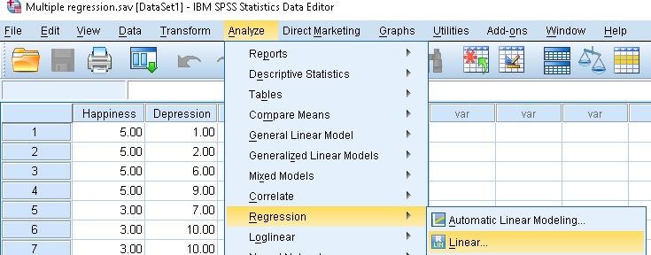
Choose Analyze, then Regression, then Linear. Row 1 of the data file reads Happiness 5.00 and Depression 1.00 behind the open menu, and the submenu lists Automatic Linear Modeling above Linear.
Check: Linear takes any number of predictors, so the entry is the same as for a model with one. The Independent(s) box, not the menu, shows how many predictors the model has.
Enter Three Predictors in One Block
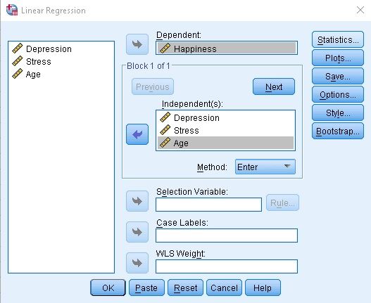
Send Happiness to the Dependent box and Depression, Stress and Age to the Independent(s) box. Block 1 of 1 and Method Enter stay as they are, and all four variables carry the scale (ruler) icon.
Watch: Enter puts all three predictors in at once. A stepwise method would pick predictors by their p-values in this sample, and the p-values and intervals of the chosen model would then look better than they are.
Set Collinearity and Residual Statistics
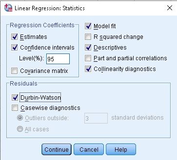
Open Statistics and tick Estimates, Confidence intervals (Level 95), Model fit, Descriptives and Collinearity diagnostics, plus Durbin-Watson in the Residuals group, then select Continue.
Tip: Collinearity diagnostics adds the Tolerance and VIF columns to the Coefficients table and a separate Collinearity Diagnostics table. The Viewer outline lists that table, but no screenshot shows it.
Request Residual Plots in the Plots Dialog
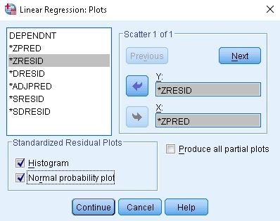
In Plots, *ZRESID goes to Y and *ZPRED to X, and Histogram and Normal probability plot are both ticked under Standardized Residual Plots. Select Continue, then OK.
Check: The pictures here cover the dialog only. The Viewer outline lists three charts, but none is shown, so nothing about the residuals can be read from these screenshots and your own output must be opened.
Check the Syntax and the Opening Tables
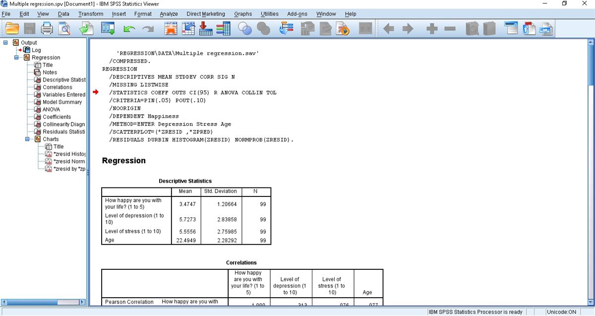
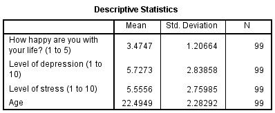
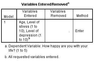
The syntax in the Log names Happiness as DEPENDENT, lists METHOD=ENTER with Depression, Stress and Age, and sets MISSING to LISTWISE. N is 99 for all four variables in Descriptive Statistics, and Variables Entered/Removed shows the three predictors going in together.
Watch: Listwise exclusion removes a whole case when any of the four variables is missing, so an N of 99 on every row of Descriptive Statistics is the check that no case was lost. Compare it with the Data Editor.
Read the Model Summary and the ANOVA Table
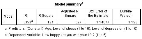
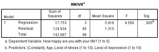
Model Summary prints R .353, R Square .124, Adjusted R Square .097, Std. Error of the Estimate 1.14677 and Durbin-Watson 1.193. ANOVA gives F(3, 95) = 4.500, p = .005 for the model.
Watch: A significant F says that the three predictors together fit better than none, not that each one matters. Only the Coefficients table shows which row does the work, and here it is Depression.
Read the Coefficients Table
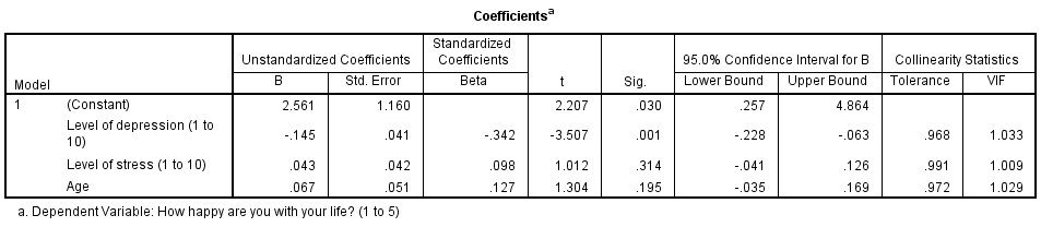
Each row gives B, Std. Error, Beta, t, Sig., the 95% interval for B, Tolerance and VIF. Depression: B -.145, Beta -.342, p = .001. Stress: B .043, p = .314. Age: B .067, p = .195. (Constant) is 2.561.
Tip: Each B compares cases that match on the other two predictors. Depression’s -.145 is therefore not the -.133 that a model with Depression alone gives (computed outside SPSS), because Stress and Age are in the model.
READING THE OUTPUT
Reading Tolerance, VIF and Durbin-Watson in the Output
Read the table one row at a time: a value from the SPSS output, the figure it takes in the video example, and how to read the same value in your data.
| Output value | In the example | How to read it |
|---|---|---|
| Mean and Std. Deviation | Happiness 3.4747 and 1.20664, Depression 5.7273 and 2.83858, Stress 5.5556 and 2.75985, Age 22.4949 and 2.28292 | The mean and spread of the four variables, each on N = 99 cases |
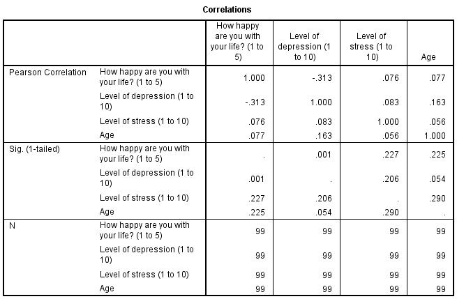
| Pearson Correlation and Sig. (1-tailed) | Happiness with Depression -.313 and .001 | The correlations with the outcome and one-sided p-values. Two-sided values are twice as large, so .001 becomes about .002 |
| R, R Square and Adjusted R Square | .353, .124 and .097 | R is the correlation of observed with predicted happiness, and R Square the share of its variance the three predictors account for in this sample |
| Durbin-Watson | 1.193 | Compares each residual with its neighbor in the file. Values near 2 fit no first-order link, and lower values point to a positive one |
| F and Sig. in ANOVA | 4.500 and .005 | Tests the three predictors together against a model with none, on 3 and 95 df |
| B and 95% Confidence Interval | Depression -.145, -.228 to -.063 | The average difference in happiness per depression point among cases matching on the other predictors. Stress and Age intervals include zero |
| Beta | -.342, .098 and .127 | The slopes in standard deviation units, in the order Depression, Stress and Age. They remove the units but not the uncertainty |
| Tolerance and VIF | .968 and 1.033, .991 and 1.009, .972 and 1.029 | Collinearity Statistics for Depression, Stress and Age in turn. FAQ 2 converts them into shares of overlap, and FAQ 3 weighs the usual cut-offs |
COMMON MISTAKES
Slips With Codes, Betas and Durbin-Watson in the Model
Here are six mistakes made with this multiple regression in the data, the dialogs, the output or the write-up, each with a short way to avoid it.
Beta Compared as Importance The Betas of -.342, .098 and .127 put the slopes in standard deviation units, but their size depends on the sample's spread and on the other predictors. Ranking predictors by Beta without intervals overstates what the data show.
Predictors Dropped on p Alone The intervals for Stress, -.041 to .126, and Age, -.035 to .169, span slopes from just below zero to clearly above it. Dropping them changes the other coefficients and does not show that they have no effect.
Pair Correlations Used Alone Correlations of .083, .163 and .056 among the predictors are low, but a predictor can be close to a combination of two others while every pair looks harmless. Tolerance, VIF and the Collinearity Diagnostics table cover that case.
Durbin-Watson Read as a Pass Mark A value of 1.193 is below 2, and a rule that accepts 1 to 3 does not make it harmless. Neighboring residuals in the file correlate at about .40 (computed outside SPSS), so ask if rows follow a class or time order.
R Squared Taken at Face Value R squared is .124 and adjusted R squared .097. R squared cannot fall when a predictor is added, so the adjusted value, which allows for three predictors in 99 cases, is the fairer summary of fit.
Category Codes Entered as Numbers A variable such as department coded 1, 2 and 3 in the Independent(s) box fits one slope across the codes, as if the steps were equal. Categories need dummy variables, and the video's three predictors are all scores or years.
If you have already run this test, Independent Statistical Review has an OnlineSPSS statistician check the predictors, the VIF values and the wording against your output.
SOURCES
Sources and Further Reading
Every entry below supports a point made on this page. Read the short line beneath it to see what it is worth reading for.
O'Brien, R. M. (2007). A caution regarding rules of thumb for variance inflation factors. Quality & Quantity, 41(5), 673-690. DOI: 10.1007/s11135-006-9018-6
Read this for why VIF cut-offs need context beyond the number.
Ernst, A. F., & Albers, C. J. (2017). Regression assumptions in clinical psychology research practice: A systematic review of common misconceptions. PeerJ, 5, Article e3323. DOI: 10.7717/peerj.3323
Read this for why the conditions concern residuals, not variables.
FREQUENTLY ASKED QUESTIONS
Menus, Predictor Overlap and VIF Cut-Offs in the Example
Four questions on this multiple regression are answered here: an SPSS screen that differs from the video, the method, the example figures and the write-up.
Why does the Linear Regression dialog look different in my SPSS?
The video was recorded in an older release of IBM SPSS Statistics. IBM’s release 30 page for the Statistics dialog also lists Selection criteria (AIC, Amemiya’s PC, Mallows’ Cp and SBC), shown in the Model Summary table when ticked. The dialog in the video offers no such choice, and its Model Summary has no extra columns.
How much of Depression overlaps with Stress and Age?
Tolerance is 1 minus the R squared from regressing a predictor on the others, so .968 means about 3% of Depression overlaps with Stress and Age. VIF is its reciprocal, 1.033, so the variance of B is about 3% larger than with uncorrelated predictors. Stress and Age overlap with the other predictors by about 1% and 3%, with Tolerance .991 and .972.
Is a VIF below 10 a safe cut-off for collinearity?
A VIF of 10 or 5 is often quoted as a limit, but such thresholds must be judged with other factors that influence the variance of a coefficient, such as the sample size and the spread of the predictor (O’Brien, 2007). Here every VIF is close to 1, so no common rule flags a predictor, and the width of each interval matters more.
How are adjusted R squared = .097 and B = -.145 written up?
Name the model, the fit, the test and the coefficient with its interval. Depression, stress and age explained R squared = .124 (adjusted .097) of the variance in happiness in 99 cases, F(3, 95) = 4.50, p = .005. Depression was the only predictor with an interval excluding zero, B = -.145, 95% CI [-.228, -.063], p = .001, among cases matching on stress and age.
NEXT STEP
Need a Multi-Predictor Model
Run or Checked?
OnlineSPSS is a statistical consultancy for researchers. Share your design and dataset, and a statistically trained Research Coordinator reviews it. The scope and one fixed project fee are confirmed before work begins.
No Commitment Required
Strictly Confidential
Fixed Project Fee
In-House PhD-Level Statisticians
Same-Day Response
Serving Researchers Since 2014