
Independent Samples t-Test in SPSS
Video Walkthrough of a Worked Example
This independent samples t-test in SPSS video runs one worked example, wage by gender, from the Compare Means menu to the output. The text below adds the checks the data need, the row to read and the mean difference with its 95% confidence interval.
WATCH THE VIDEO
Independent Samples t-Test in SPSS, Start to Finish
Decide which row of the SPSS output to report before the output is examined. The Welch row, labeled Equal variances not assumed, is the sound default for two independent groups: it keeps its error rate when the variances differ and loses little when they do not (Delacre et al., 2017), while choosing a row after Levene’s test can distort the error rate of the final test (Zimmerman, 2004). In this example the two rows agree closely.
IN SHORT
What the Video Shows in Brief
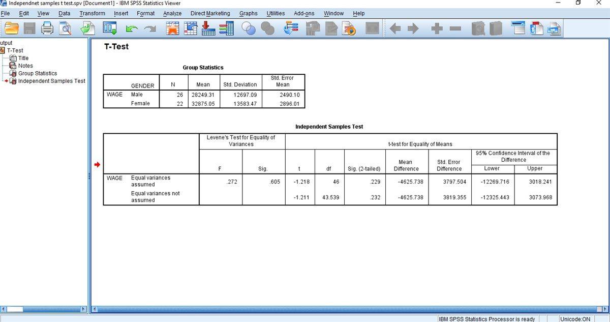
In this independent samples t-test in SPSS video, annual wage is compared between 26 male and 22 female cases, with GENDER coded 0 and 1. The path is Analyze, Compare Means, Independent-Samples T Test, then Define Groups with the codes 0 and 1. In the Welch row (Equal variances not assumed), the mean difference (Male minus Female) is -4,625.74 dollars, 95% CI [-12,325.44, 3,073.97], p = .232: not statistically significant, and the interval includes zero.
BEFORE YOU RUN
What the Test Needs From Your Data
These four points cover what to check in your study design and data, and each one is settled before the analysis is run in SPSS.
Independent Groups Each case belongs to one group and is unrelated to the others, which the design settles, not a diagnostic. Two measurements on one person call for the paired test, and clustered cases (one clinic, one classroom) for a multilevel model.
A Continuous Outcome The outcome is measured on an interval or ratio scale, such as annual wage in dollars. An ordinal outcome, or one whose means are not meaningful, points to a rank-based comparison such as the Mann-Whitney U test.
Shape Within Each Group The test concerns means, so inspect each group with a histogram or boxplot, not the pooled variable. Moderate skew is tolerated at moderate group sizes (Lumley et al., 2002). Strong skew or outliers in small groups need more care.
Variances Need Not Match Equal variances are not required when the Welch row is read. Levene's test appears in the output, but choosing the row only after seeing it makes one test conditional on another. The row is decided before looking at the output.
STEP BY STEP
Running the Test in the SPSS Dialogs
The screenshots show each screen in IBM SPSS, and the numbered steps below give the menu path, the settings to choose and a check or tip for each step.
Each slide shows the SPSS screen for one step and carries its step number. The video was recorded in an older release, so labels on your screen may differ slightly.
Open the Independent-Samples Dialog
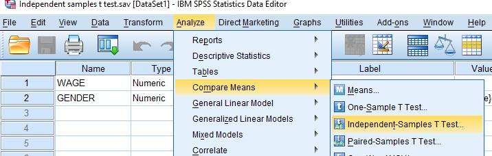
Choose Analyze, then Compare Means (Compare Means and Proportions in recent releases), then Independent-Samples T Test. The same submenu lists the One-Sample and Paired-Samples versions, so check that the independent version is the one selected.
Check: Two groups made up of different cases belong in this dialog. The same cases measured twice belong in the Paired-Samples T Test, and the choice is made from the design.
Move the Outcome to Test Variable(s)
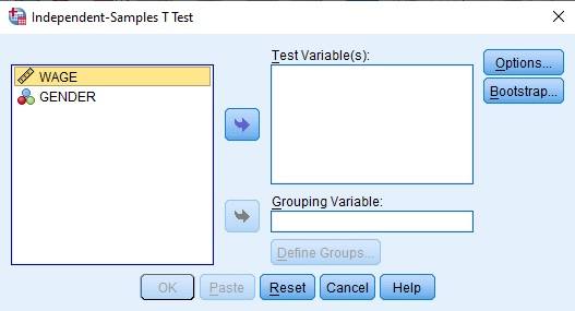
Select the continuous outcome (WAGE in the example) and move it into the Test Variable(s) box with the arrow button or a double click. Several outcomes can be listed, and each gets its own t-test.
Watch: Every extra outcome is an extra comparison. List only the outcomes named in the analysis plan, so the number of tests stays small and the multiplicity can be handled.
Add the Grouping Variable
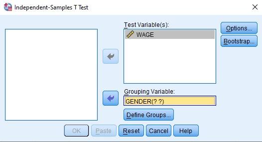
Move the two-category variable (GENDER in the example) into the Grouping Variable box. It appears as GENDER(? ?) until the two group codes have been entered in the next steps.
Tip: The grouping variable can have more than two categories in the data. Define Groups then picks the two to compare, and cases outside those two codes are left out of the test.
Check How the Groups Are Coded
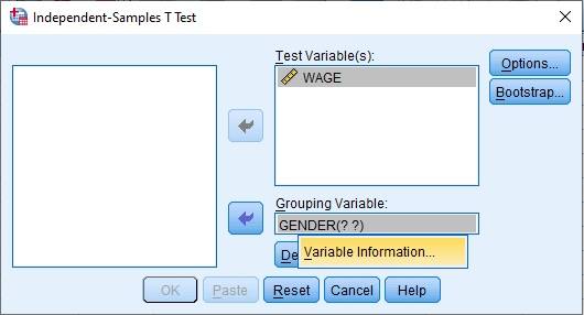
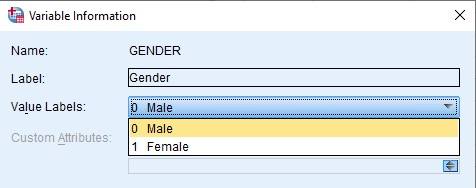
Right-click the variable in the Grouping Variable box and choose Variable Information. In the example the value labels show 0 as Male and 1 as Female. Close the window to return to the dialog.
Check: Read the value labels before typing any code. A reversed label is easy to miss, and it would flip the direction of the mean difference in the output without any warning.
Define the Two Groups
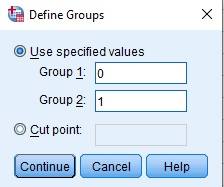
Select Define Groups, keep Use specified values, enter 0 for Group 1 and 1 for Group 2, then select Continue and OK. The Options button holds the confidence level, which is 95% by default.
Watch: The mean difference is Group 1 minus Group 2, here Male minus Female, so the negative value means the female mean is higher. Name that order in the write-up.
Open the Output and Check the Counts
The Viewer shows a T-Test heading with Title, Notes, Group Statistics and Independent Samples Test. Before reading any test result, confirm that the N in each group matches the cases you expect.
Check: Cases with a missing outcome or a missing group code drop out of the test without a message. A group N below the number recruited is the first sign that this has happened.
READING THE OUTPUT
How to Read the Two SPSS Output Tables
Each row of the table names one value in the SPSS output, gives its figure in the video example and says how to read it for your own data.
| Output value | In the example | How to read it |
|---|---|---|
| N | Male 26, Female 22 | Valid cases per group. Together they give the df of 46 (48 cases minus 2) |
| Mean and Std. Deviation | Male 28249.31 (12697.09), Female 32875.05 (13583.47) | Group means and spread in dollars per year. Report the SD, not the Std. Error Mean |
| Levene’s Test, F and Sig. | .272 and .605 | A check on equal variances, shown for information. A large p is not proof that the variances are equal |
| t and df | -1.218 and 46 (assumed), -1.211 and 43.539 (not assumed) | The Welch row has fractional df. Both rows are printed, and one is reported |
| Sig. (2-tailed) | .229 and .232 | Two-sided p for the row reported. It does not measure how large the difference is |
| Mean Difference | -4625.738 in both rows | Male minus Female, because Male was entered as Group 1 |
| Std. Error Difference | 3797.504 and 3819.355 | Uncertainty of the difference, slightly larger in the Welch row here |
| 95% CI of the Difference | -12269.716 to 3018.241, and -12325.443 to 3073.968 | The differences compatible with the data. Zero is inside, and so are differences of either sign |
COMMON MISTAKES
Slips to Avoid With This Test
These six mistakes arise in the data setup, the SPSS dialogs, the output or the write-up, and each comes with a short note on how to avoid it.
Group Codes That Match No Cases Entering 1 and 2 in Define Groups when the data use 0 and 1 leaves a group empty, and SPSS returns a warning in place of the test. Type the codes shown in Variable Information.
Reading p Above .05 as No Difference A non-significant result does not show that the groups are equal. The interval for the mean difference shows which differences remain compatible with the data.
Testing the Sample Means The two sample means in the output do differ. The hypothesis concerns the population means, and the test asks whether the observed gap is compatible with sampling variation.
Uneven N Across Several Outcomes With several test variables, the default under Options excludes cases analysis by analysis, so each t-test can rest on a different N. Choose listwise exclusion when the tests must share one sample.
Keeping No Syntax or Output File A screenshot cannot be rerun or checked. Select Paste instead of OK to save the command as syntax, and keep the .spv output file with the dataset, so the test can be reproduced and reviewed.
Testing Normality on the Pooled Outcome What matters is the shape of the outcome within each group, judged with the group sizes. A single normality test on the whole variable answers a different question.
If you have already run this test, Independent Statistical Review has an OnlineSPSS statistician check the row, the interval and the wording against your output.
SOURCES
Sources and Further Reading
The sources below support statements made on this page, and the line under each entry says what to read it for.
Delacre, M., Lakens, D., & Leys, C. (2017). Why psychologists should by default use Welch's t-test instead of Student's t-test. International Review of Social Psychology, 30(1), 92-101. DOI: 10.5334/irsp.82
Read this for the case for reporting the Welch row by default.
Zimmerman, D. W. (2004). A note on preliminary tests of equality of variances. British Journal of Mathematical and Statistical Psychology, 57(1), 173-181. DOI: 10.1348/000711004849222
Read this to see why choosing a row after Levene's test is risky.
Lumley, T., Diehr, P., Emerson, S., & Chen, L. (2002). The importance of the normality assumption in large public health data sets. Annual Review of Public Health, 23(1), 151-169. DOI: 10.1146/annurev.publhealth.23.100901.140546
Read this for how far the t-test tolerates departures from normality.
FREQUENTLY ASKED QUESTIONS
Menus, Distributions and Effect Size in the Example
These answers explain why the SPSS screens may look different from the video, then take up the method, the example figures and how to write the result up.
Why does my SPSS menu look different from the video?
The video was recorded in an older release of IBM SPSS Statistics. In recent releases the submenu reads Compare Means and Proportions, and the Independent-Samples T Test dialog adds an option to estimate effect sizes. The Test Variable(s) box, the grouping variable, Define Groups and the two rows of the output work as shown in the video.
Must the outcome be normally distributed?
The condition concerns the distribution within each group, and approximate shape is usually enough at moderate group sizes. Wages are often right-skewed, so inspect each group with a histogram or boxplot. With small groups and strong skew or extreme outliers, a rank-based test or a robust approach may fit better.
Where do I find Cohen's d for this test in SPSS?
Recent releases print an Independent Samples Effect Sizes table when Estimate effect sizes is ticked in the dialog, and older releases, as in the video, need d computed from the group means and SDs. For this example the pooled SD is about 13,109 dollars, so d is about -0.35 (Male minus Female), with a wide interval at these group sizes.
How would the example result be reported?
With both group summaries, the mean difference, its interval and a named effect size. Male (M = 28,249.31, SD = 12,697.09, n = 26) and Female (M = 32,875.05, SD = 13,583.47, n = 22): mean difference -4,625.74, 95% CI [-12,325.44, 3,073.97], Welch t(43.54) = -1.21, p = .232, Cohen’s d = -0.35. The pooled row gives the same conclusion.
NEXT STEP
Need This Comparison
Run or Checked on Your Data?
OnlineSPSS is a statistical consultancy for researchers. Share your design and dataset, and a statistically trained Research Coordinator reviews it. The scope and one fixed project fee are confirmed before work begins.
No Commitment Required
Strictly Confidential
Fixed Project Fee
In-House PhD-Level Statisticians
Same-Day Response
Serving Researchers Since 2014