
Friedman Test in SPSS
Video Walkthrough of a Worked Three-Occasion Example
This Friedman test in SPSS video asks whether the math scores of 23 people differ across three occasions in K Related Samples. The page adds why Chi-Square is Friedman's statistic, what mean ranks near 2 show and where Kendall's W fits beside it.
WATCH THE VIDEO
Friedman Test in SPSS, Start to Finish
Keep the question on ranks within each person. Friedman’s test ranks one person’s three scores against each other and compares the mean ranks (Friedman, 1937), so the medians in the first table describe the data but are not what is tested. Here p = .276 is no evidence of a difference, which is not the same as scores that stayed put.
IN SHORT
What the Video Shows in Brief
In this Friedman test in SPSS video, the math scores of 23 people are compared before training, after the first training and after the second training. The path is Analyze, Nonparametric Tests, Legacy Dialogs, K Related Samples, with Friedman ticked and Quartiles requested. SPSS prints Chi-Square = 2.571, df = 2 and Asymp. Sig. = .276: not statistically significant.
BEFORE YOU RUN
Checks on Repeated Scores Before K Related Samples
These four points cover what to check in your study design and data, and each one is settled before the analysis is run in SPSS.
One Row per Person Each row holds one person with a score in each of three columns, and the design settles this. A person with any score missing drops out of the test, and people nested in classes call for a model for clustered data.
Ordering Inside Each Person Only each person's own ordering of the three scores is used. That suits an ordinal outcome, or a score whose means are hard to defend, and the test is not a test of medians.
A Fixed Order of Occasions The occasions always came in the same order, with no comparison group. A rise or fall across them mixes training with practice and time, so the result describes change across occasions.
The Chi-Square Approximation The p-value comes from a chi-square approximation that SPSS adjusts for ties, and one person here has tied scores (98, 98 and 68). With few people, ask for the exact p-value in the Exact dialog where licensed.
STEP BY STEP
Setting Up Tests for Several Related Samples
The screenshots show each screen in IBM SPSS, and the numbered steps below give the menu path, the settings to choose and a check or tip for each step.
Every slide pictures the SPSS screen for a single step and is numbered to match it. Labels in your version may differ a little, as the video comes from an older release.
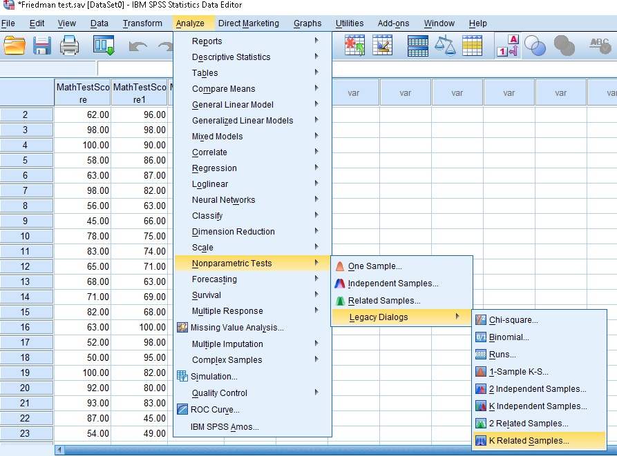
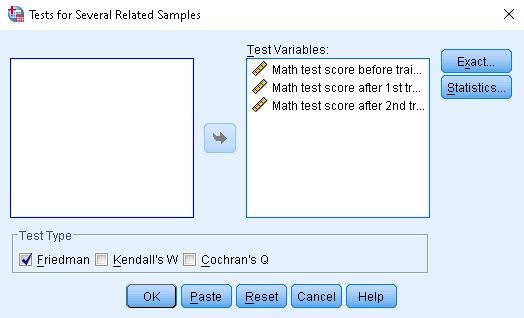
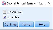
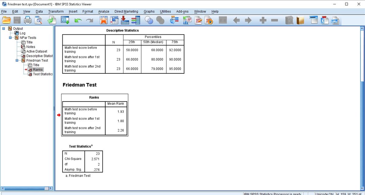
Open the K Related Samples Dialog
Choose Analyze, then Nonparametric Tests, then Legacy Dialogs, then K Related Samples. A window titled Tests for Several Related Samples opens, listing the variables at its left.
Check: The entry above it, 2 Related Samples, takes only two columns. Three occasions of the same people belong in K Related Samples, since three separate pair tests would be three unadjusted tests.
Move the Three Scores Into Test Variables
Select the three score variables, labeled before training, after 1st training and after 2nd training, and move them into the Test Variables box with the arrow button. Under Test Type, Friedman is ticked.
Tip: Ticking Kendall’s W as well would add a block with W beside the same chi-square. Cochran’s Q is built for yes/no outcomes, so it has no use for scores.
Request Quartiles Under Statistics
Select Statistics, tick Quartiles, leave Descriptive unticked, then Continue and OK. The Exact button beside Statistics is not used, which is why the output prints only Asymp. Sig.
Watch: Quartiles only describe each column, and the test never uses them. Leaving Descriptive unticked keeps the first table to N and three percentiles per occasion.
Open the Viewer and Count 23 People
The Viewer lists NPar Tests with Title, Notes, Active Dataset and Descriptive Statistics, then a Friedman Test branch holding Ranks and Test Statistics. Confirm that N is 23 in the first and the last table.
Check: The test uses only people who have all three scores. An N below the number of people in the file means a missing score somewhere, and Descriptive Statistics can still show a larger N for one occasion.
Read the Descriptive Statistics Table
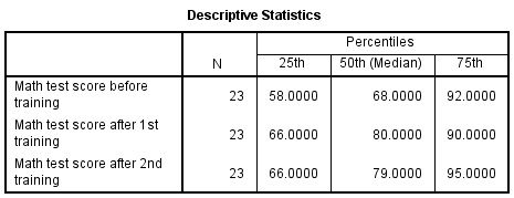
Each occasion gets an N and three percentile columns: 25th, 50th (Median), 75th. The medians are 68, 80 and 79, with quartiles from 58 to 92, from 66 to 90 and from 66 to 95.
Watch: The median before training is 12 points below the one after the first training, yet its mean rank is higher (1.93 against 1.80). Ranks are taken inside each person, so column medians and mean ranks need not agree.
Read the Ranks Table and Mean Ranks
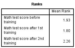
Ranks prints one Mean Rank per occasion: 1.93 before training, 1.80 after the first and 2.26 after the second. SPSS ranks each person’s three scores from 1 to 3 and averages those places over the 23 people.
Check: Three mean ranks must add up to 6 apart from rounding (1.93 + 1.80 + 2.26 = 5.99). A different total means the test did not rest on three occasions.
Read the Test Statistics Table
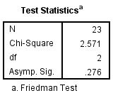
The table prints N = 23, Chi-Square = 2.571, df = 2 and Asymp. Sig. = .276, and footnote a names the Friedman Test. The df is the number of occasions minus 1.
Tip: Sig. prints as .276 and not as 0.276, and a very small p appears as .000. In a write-up the first is p = .276 and the second is p < .001.
READING THE OUTPUT
Reading Mean Ranks and Friedman's Chi-Square
For each value it lists from the SPSS output, the table gives the example figure from the video and explains how to read it in your own data.
| Output value | In the example | How to read it |
|---|---|---|
| N | 23 | People with all three scores, so all 23 rows are complete. Test Statistics repeats it, and N is quoted beside the statistic |
| 25th, 50th (Median), 75th | Before 58, 68, 92; after 1st 66, 80, 90; after 2nd 66, 79, 95 | Spread of each column in score points. They describe the scores and do not enter the test |
| Mean Rank | 1.93, 1.80 and 2.26 | Average place of each occasion within people, on a scale from 1 to 3, with tied scores sharing a place. Equal occasions would sit near 2 |
| Chi-Square | 2.571 | Friedman’s statistic, adjusted for ties. It is not the chi-square test of a crosstab |
| df | 2 | Three occasions minus 1 |
| Asymp. Sig. | .276 | A p-value computed from the chi-square distribution with 2 df. It says nothing about the size of any difference |
| Footnote a | Friedman Test | Names the test. Check it against the analysis plan before the figures are quoted or copied out of the Viewer |
| Kendall’s W (not printed here) | .056 | The chi-square over N times the df, 2.571 / (23 x 2). It gauges agreement among the rankings, ranging from 0 to 1 |
COMMON MISTAKES
Slips With Test Variables and the Chi-Square Label
Six mistakes with the Friedman test are set out below. Each comes from the data setup, dialogs, output or write-up, with a short note on avoiding it.
Chi-Square Reported as a Crosstab Test The Chi-Square row is Friedman's statistic, not the test of a table. Write it as chi-square(2, N = 23) = 2.57 and name the Friedman test in the sentence, so no reader looks for a contingency table.
Long-Format Scores in the Dialog Each variable in the Test Variables box is one occasion. Scores stacked in a single column with a Time code must first be spread across three columns, one row per person.
A Stray Variable in Test Variables Every variable in the box becomes an occasion. A fourth column such as an ID turns df 2 into 3 and changes every rank, so check that df equals the occasions minus 1 and that three scores are listed.
Follow-Up Pairs Run Unadjusted After a Friedman test with p = .276, three Wilcoxon tests on the pairs can still show one p below .05 by chance. Follow-ups belong after a significant result, with p-values adjusted for the three pairs.
Sample Size Given as 69 Scores The N in Test Statistics is 23 people, not the 69 scores behind the three mean ranks. Quoting 69 as the sample size presents repeated scores as independent people and overstates the evidence.
Mean Ranks Quoted as Mean Scores A mean rank of 1.93 is an average place between 1 and 3, not a math score. Label mean ranks as ranks and medians in score points, so no reader takes 1.93 for points on the test.
If you have already run this test, Independent Statistical Review has an OnlineSPSS statistician check the ranks, the pairs and the wording against your output.
SOURCES
Sources and Further Reading
Statements on this page draw on the literature listed below, and a line under each entry says what it is worth reading for.
Friedman, M. (1937). The use of ranks to avoid the assumption of normality implicit in the analysis of variance. Journal of the American Statistical Association, 32(200), 675-701. DOI: 10.1080/01621459.1937.10503522
Read this for the ranking approach behind the test.
Kendall, M. G., & Babington Smith, B. (1939). The problem of m rankings. The Annals of Mathematical Statistics, 10(3), 275-287. DOI: 10.1214/aoms/1177732186
Read this for Kendall's coefficient of concordance, W.
FREQUENTLY ASKED QUESTIONS
Menus, Follow-Ups and Kendall's W in the Example
Each question below concerns this analysis in SPSS: why a screen may differ from the video, a point of method, a figure in the example or the write-up.
Why does the Tests for Several Related Samples dialog look different in my SPSS?
The video was recorded in an older release of IBM SPSS Statistics. Release 30 keeps K Related Samples where the video shows it, under Analyze, Nonparametric Tests, Legacy Dialogs, according to IBM’s page, which lists Friedman, Kendall’s W and Cochran’s Q as test types and quartiles under Statistics. The Test Variables box and the three output tables work as shown.
Which follow-up comparisons fit a Friedman test, and are any needed here?
None is needed here, because the overall test is not significant. After a significant result, the Nonparametric Tests branch has a Related Samples dialog whose pairwise comparisons carry p-values adjusted for the three pairs, and Wilcoxon signed-rank tests with a Bonferroni or Holm adjustment are the other common route. The legacy dialog prints none.
Does SPSS print Kendall's W beside the Friedman chi-square of 2.571?
Only when Kendall’s W is ticked under Test Type, which the video leaves off. W gauges how closely the individual rankings agree (Kendall & Babington Smith, 1939), and here it is 2.571 / (23 x 2) = .056, close to zero. With 23 people the estimate is imprecise, so quote it with N.
How is a Friedman chi-square of 2.571 for 23 people worded?
With the statistic, df, N and p, plus the medians. The Friedman result was not statistically significant, chi-square(2, N = 23) = 2.57, p = .276, W = .06, with medians of 68 (before training), 80 (after the first) and 79 (after the second) and mean ranks of 1.93, 1.80 and 2.26.
NEXT STEP
Need Three-Occasion Scores
Run or Checked?
OnlineSPSS is a statistical consultancy for researchers. Share your design and dataset, and a statistically trained Research Coordinator reviews it. The scope and one fixed project fee are confirmed before work begins.
No Commitment Required
Strictly Confidential
Fixed Project Fee
In-House PhD-Level Statisticians
Same-Day Response
Serving Researchers Since 2014