
Descriptive Statistics in SPSS
Video Walkthrough of a Worked Example
This descriptive statistics in SPSS video summarizes 48 cases, with four categorical variables in Frequencies and wage and age in Descriptives. The page adds how to match a summary to a variable type, what Valid Percent leaves out and which figures to read.
WATCH THE VIDEO
Descriptive Statistics in SPSS, Start to Finish
Choose the summary for each variable from its type before any output is requested: counts and percentages for categories, the mean and standard deviation for a roughly symmetric scale variable. Report the standard deviation, not the standard error, beside the mean, because the standard error expresses how precisely the mean is estimated and not the spread of the data (Altman & Bland, 2005). In this example the two procedures divide the six variables cleanly.
IN SHORT
What the Video Shows in Brief
In this descriptive statistics in SPSS video, 48 cases are summarized in two runs: Frequencies for four categorical variables and Descriptives for two scale variables. The paths are Analyze, Descriptive Statistics, Frequencies and Analyze, Descriptive Statistics, Descriptives. Wage has a mean of 30,369.44 dollars (SD = 13,176.48, range 10,111 to 58,999) and age a mean of 36.10 years (SD = 7.55); 23 cases work in manufacturing and 25 in construction.
BEFORE YOU RUN
Matching Each Summary to the Variable Type
Before you open the SPSS dialogs, the four points below need an answer from your study design and from the data themselves.
Variable Type Sets the Summary Counts and percentages describe categories, and the mean and standard deviation describe a scale variable. An ordinal variable such as job responsibility takes counts, or the median and quartiles.
Cases and Missing Values Every table rests on the cases that have a value. The output reports valid and missing counts for each variable, and Valid Percent leaves missing cases out of its base, so read N before any percentage.
Shape Before the Mean A mean and standard deviation summarize a roughly symmetric scale variable well. Skewed values or outliers call for the median and quartiles beside them, so look at the distribution of each one.
A Description, Not a Test These tables describe the cases in the file and test no hypothesis, so no p-value appears. A statement about a wider population needs an interval or a test, which come in a later analysis.
STEP BY STEP
Running Frequencies and Descriptives
The screenshots come from IBM SPSS. Read them alongside the numbered steps below: the menu path, the settings to choose and a check or tip for every step.
The slides follow the step numbers, each one showing the SPSS screen for that step. The video was made in an older release, so some labels on your screen may differ.
Open the Frequencies Dialog
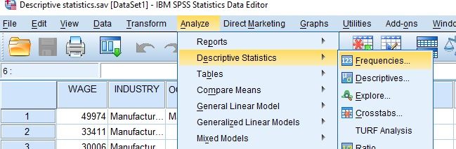
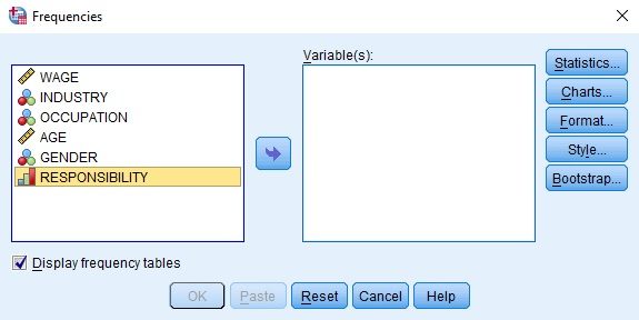
Choose Analyze, then Descriptive Statistics, then Frequencies. The dialog opens with all six variables in the left list and an empty Variable(s) box.
Check: Categorical variables go to Frequencies and scale variables to Descriptives. The icon beside each variable name in the dialog shows how SPSS has stored its measurement level.
Move the Categorical Variables
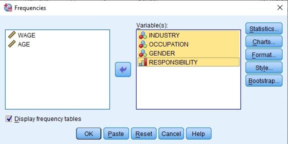
Select INDUSTRY, OCCUPATION, GENDER and RESPONSIBILITY and move them into the Variable(s) box with the arrow button. Keep Display frequency tables ticked. WAGE and AGE stay in the list.
Watch: The Format button sets the order of the categories in each table. Keep ascending values for an ordinal variable such as RESPONSIBILITY, so its Cumulative Percent follows the scale.
Request Bar Charts
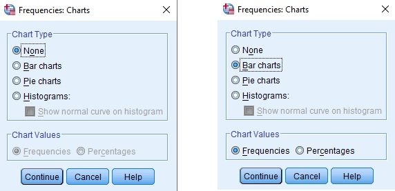
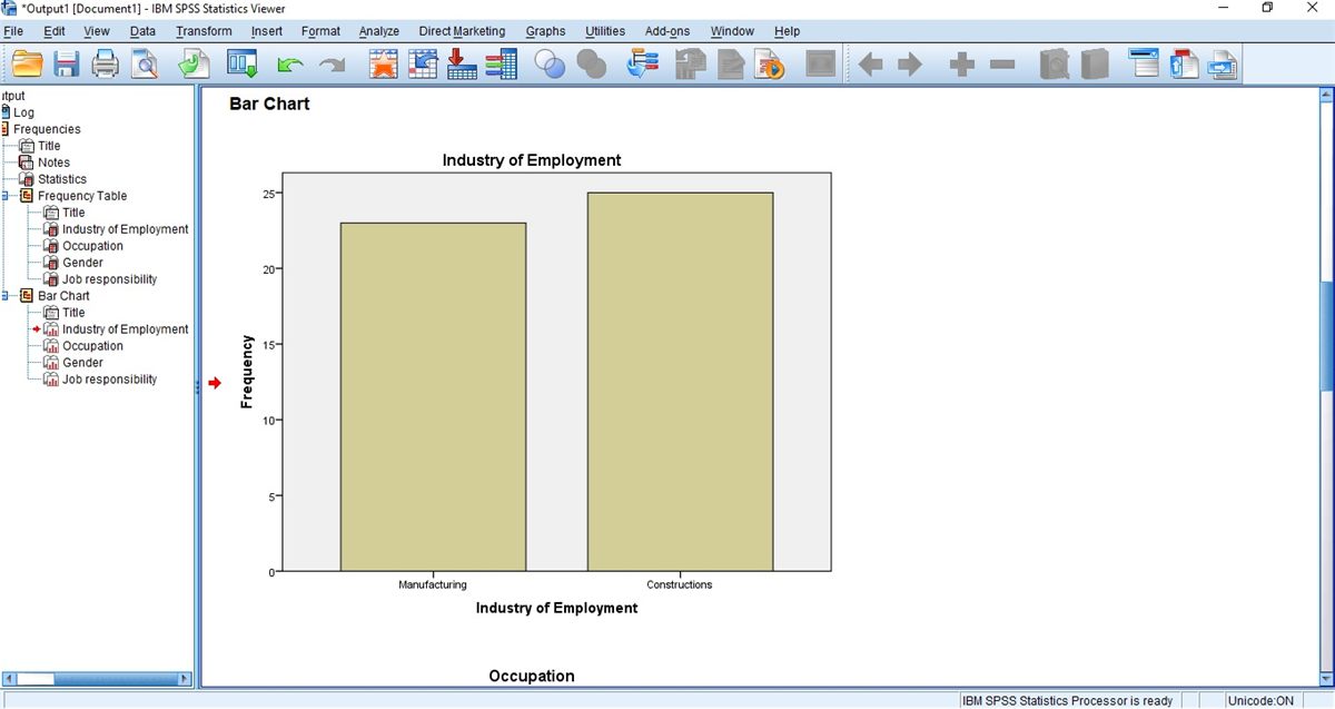
Select Charts, choose Bar charts with Chart Values set to Frequencies, then select Continue and OK. The Chart Type shows None until a type is chosen, and the run then prints tables only.
Tip: Bar charts suit nominal and ordinal variables. A histogram belongs to a scale variable, and the same Charts button offers it, with an optional normal curve.
Read the Frequencies Output
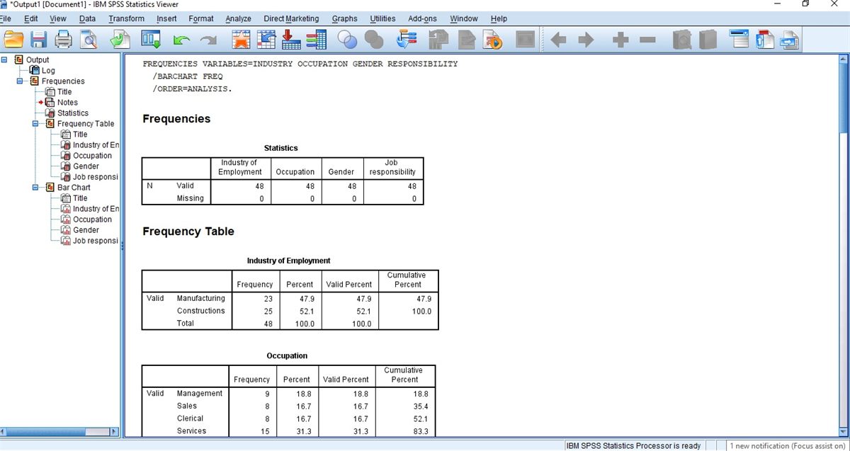
The Viewer shows the command, a Statistics table with the valid and missing N, one Frequency Table for each variable and then the bar charts. Confirm that Valid is 48 for each variable before reading a percentage.
Check: Percent uses all cases, and Valid Percent only the cases with a value. They agree here because Missing is 0, and they part company as soon as a variable has gaps.
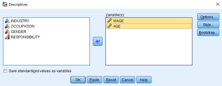
Open the Descriptives Dialog
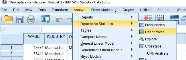
Choose Analyze, then Descriptive Statistics, then Descriptives. This dialog summarizes scale variables with numbers only: it prints no frequency table and draws no chart.
Check: Descriptives accepts any numeric variable, including a coded category such as GENDER, and prints a mean for it without a warning. The choice of variables rests with you.
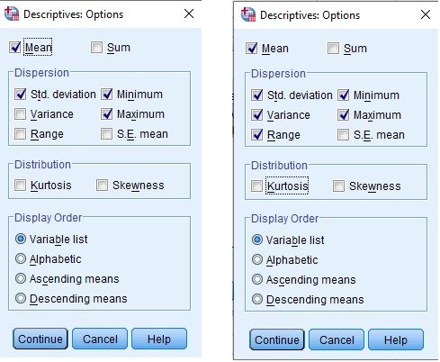
Choose the Variables and Options
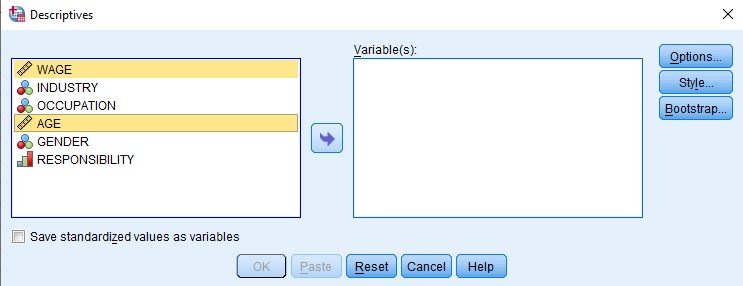
Move WAGE and AGE into the Variable(s) box, then select Options. Mean, Std. deviation, Minimum and Maximum are ticked by default, and the video adds Variance and Range before Continue and OK.
Watch: Save standardized values as variables, at the foot of the dialog, adds a z-score column for each listed variable to the data file. Leave it unticked unless those scores are needed.
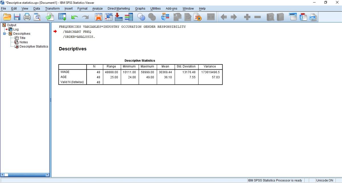
Read Range, Mean and SD for Each Variable
The table lists N, Range, Minimum, Maximum, Mean, Std. Deviation and Variance for each variable. Valid N (listwise) at the bottom counts the cases that have a value on every listed variable.
Check: Compare Minimum and Maximum with the values the variable can take. A wage of zero or an age of 240 would show up here before it distorts the mean.
READING THE OUTPUT
Reading the Frequency and Descriptive Tables
Read the table one row at a time: a value from the SPSS output, the figure it takes in the video example, and how to read the same value in your data.
| Output value | In the example | How to read it |
|---|---|---|
| N, Valid and Missing | 48 and 0 for each categorical variable | Cases with a value on that variable. Read it before any percentage |
| Frequency and Percent | Manufacturing 23 (47.9), Constructions 25 (52.1) | Count per category and its share of all cases, which adds to 100 before rounding |
| Valid Percent | 47.9 and 52.1, equal to Percent | Share among cases with a value. It differs from Percent only when values are missing |
| Cumulative Percent | Job responsibility: small 35.4, medium 72.9, high 100.0 | A running total in category order. It has meaning for ordinal variables, not nominal ones |
| Minimum, Maximum and Range | Wage 10111.00, 58999.00 and 48888.00; Age 24.00, 49.00 and 25.00 | The extremes and their gap, in the units of the variable. Check them against possible values |
| Mean | Wage 30369.44, Age 36.10 | The arithmetic average in the variable’s own units. Extreme values pull it |
| Std. Deviation | Wage 13176.48, Age 7.55 | Spread around the mean in the same units. Report this, not the standard error |
| Variance | Wage 173619496.5, Age 57.03 | The squared SD, in squared units. The SD is the figure to read |
COMMON MISTAKES
Slips With Percentages, Labels and Codes
The six slips below happen while setting up the data, working in the SPSS dialogs, reading the output or writing up, and each has a note on prevention.
A Scale Variable in Frequencies Putting WAGE in the Frequencies dialog prints a table with a row for nearly every case and no useful summary. Use Descriptives for the mean and SD of a scale variable.
Percents That Add to 100.2 Occupation's printed percents, 18.8, 16.7, 16.7, 31.3 and 16.7, add to 100.2 because each one is rounded. Report them as printed and note the rounding, rather than changing one figure to force 100.
Looking for the Median in Descriptives The Descriptives table prints no median or quartiles, which a skewed wage variable needs beside its mean. Run Frequencies with its Statistics button, or Explore, to obtain them.
Value Labels Left Undefined Frequencies prints the value labels stored in the data file. Industry shows Manufacturing and Constructions because they are defined there, and an undefined code prints as a bare number. Define the labels before the run.
Decimals the Output Never Printed The output gives 47.9 and 52.1. Writing 47.90% and 52.10% adds a precision the table does not hold, so each percentage is copied at the one decimal SPSS printed.
Missing Codes Left in as Values A code such as 99 for an unknown age is read as a real value until Variable View declares it missing. Until then, it enters the mean and range, while N and Valid Percent look complete.
If you have already run these tables, Independent Statistical Review has an OnlineSPSS statistician check the summaries, percents and wording against your output.
SOURCES
Sources and Further Reading
Every entry below supports a point made on this page. Read the short line beneath it to see what it is worth reading for.
Altman, D. G., & Bland, J. M. (2005). Standard deviations and standard errors. BMJ, 331(7521), 903. DOI: 10.1136/bmj.331.7521.903
Read this for how the standard deviation and standard error differ.
FREQUENTLY ASKED QUESTIONS
Menus, Percentages and Variance in the Example
Questions on this descriptive analysis follow, from a screen that looks different in SPSS through the method and the video example to wording the result.
Why does the Frequencies dialog look different in my SPSS?
The video was recorded in an older release of IBM SPSS Statistics. Its menu bar still lists Direct Marketing, and the path to Frequencies is unchanged. Release 29.0.1 added a Percentiles dialog to the Descriptive Statistics submenu for quartiles or custom percentiles. The Variable(s) box and the Charts button are used as in the video.
Why are Percent and Valid Percent identical in the output?
Percent divides each count by all 48 cases, and Valid Percent divides it by the cases that have a value. The Statistics table shows 0 missing for all four variables, so the two columns match. With missing values, Valid Percent rises above Percent and the table needs a note on its base.
Why is the variance of wage so much larger than the SD?
The variance is the squared standard deviation, so it is in squared dollars: 173,619,496.5 for wage against an SD of 13,176.48 dollars. Age shows the same pattern on a smaller scale, 57.03 against 7.55 years. Report the SD, which is in the units of the variable, and keep the variance for calculations that need it.
How are the industry shares and the wage mean and SD written down?
With a count and percentage for each category and a mean and SD for each scale variable, with n. Industry: manufacturing 23 (47.9%), construction 25 (52.1%). Wage: M = 30,369.44, SD = 13,176.48, range 10,111 to 58,999. Age: M = 36.10, SD = 7.55, range 24 to 49 (n = 48). No p-value belongs here, since no hypothesis was tested.
NEXT STEP
Need a Sample Description
Run or Checked on Your Data?
OnlineSPSS is a statistical consultancy for researchers. Share your design and dataset, and a statistically trained Research Coordinator reviews it. The scope and one fixed project fee are confirmed before work begins.
No Commitment Required
Strictly Confidential
Fixed Project Fee
In-House PhD-Level Statisticians
Same-Day Response
Serving Researchers Since 2014