
One-Way ANOVA in SPSS
Video Walkthrough of a Worked Annual Wage Example
This one-way ANOVA in SPSS video compares annual wage across three job responsibility groups of 96 employees, with Welch and Games-Howell ticked. The page adds why the Welch result is the default, how the two post hoc families differ and what eta squared adds.
WATCH THE VIDEO
One-Way ANOVA in SPSS, Start to Finish
Settle the choice between the classical F and the Welch result before the output is opened. The Welch result is a sound default for a one-way layout: when the variances differ it keeps the Type I error rate near its nominal level, and when they are equal it costs little power (Delacre et al., 2019), so Levene’s test is for information, not for choosing a table. In this example the classical F and the Welch test agree, and so do both post hoc methods.
IN SHORT
What the Video Shows in Brief
In this one-way ANOVA in SPSS video, annual wage is compared across three job responsibility groups: small (n = 31), medium (n = 33) and high (n = 32). The path is Analyze, Compare Means, One-Way ANOVA, with WAGE in Dependent List and RESPONSIBILITY as Factor. The Welch test gives F(2, 60.99) = 23.12 and the classical test F(2, 93) = 24.19, both p < .001, with eta squared about .34: wages differ across the groups, and the small group is lowest.
BEFORE YOU RUN
What the Factor and the Wage Groups Need Before Welch
Four points about your design and your data come first. Each of them is decided before this one-way ANOVA is run in SPSS.
Independent Groups Each employee appears in one responsibility group only, with no pairing or clustering of records. Wages of the same staff recorded three times call for repeated measures ANOVA, and employees nested in firms for a multilevel model.
A Continuous Outcome Wage in dollars has equal steps, so its group means carry meaning. Ordinal wage bands, or any outcome whose means mislead, are better compared through ranks, as the Kruskal-Wallis test does.
Shape Within Each Group Inspect wages in each group, since the pooled column mixes three distributions. A test of means tolerates moderate skew in reasonably large groups (Lumley et al., 2002), but a strongly skewed group of about 32 deserves a closer look.
Variances Need Not Match The Welch result does not require equal variances. Preliminary tests of variance often fail to detect real differences (Delacre et al., 2019), so a large Levene p is not proof that they match.
STEP BY STEP
Filling Dependent List, Factor and Post Hoc Ticks
Menu path, settings and a check or tip: the numbered steps below give all three for every step of this one-way ANOVA, with screenshots from IBM SPSS.
Every slide pictures the SPSS screen for a single step and is numbered to match it. Labels in your version may differ a little, as the video comes from an older release.
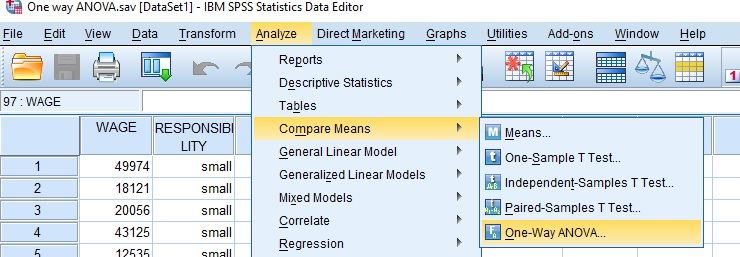
Open the One-Way ANOVA Dialog
Choose Analyze, then Compare Means (Compare Means and Proportions in recent releases), then One-Way ANOVA. The dialog opens on the variable list, with the Dependent List and Factor boxes still to fill.
Check: One grouping variable with three or more independent groups belongs in this dialog. Two groups can use the independent samples t-test, and the same cases measured repeatedly need a repeated measures model.
Set the Dependent List and the Factor
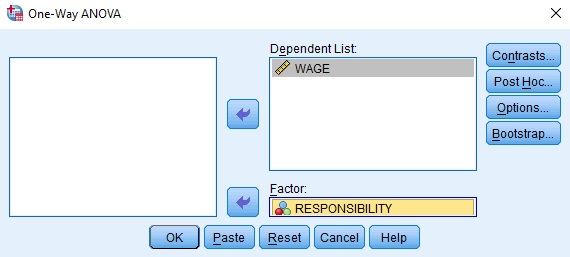
Move the continuous outcome (WAGE, labeled Annual Wages in Dollars) into Dependent List and the grouping variable (RESPONSIBILITY, coded 1 small, 2 medium, 3 high) into Factor. The Contrasts, Post Hoc, Options and Bootstrap buttons run down the right side.
Watch: Each variable added to the Dependent List is tested on its own, and no p-value is adjusted for the others. Keep the list to the outcomes in the analysis plan.
Choose the Options and Post Hoc Tests
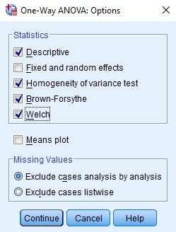
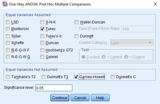
Select Options and tick Descriptive, Homogeneity of variance test, Brown-Forsythe and Welch, then Continue. Select Post Hoc, tick Tukey and Games-Howell with the level at .05, then Continue and OK.
Check: Ticking Welch and both post hoc families prints every block. Decide which F and which comparisons you report before opening the output, and name them in the write-up.
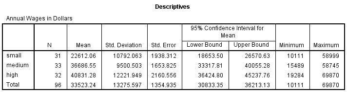
Confirm the Three Group Ns in Descriptives
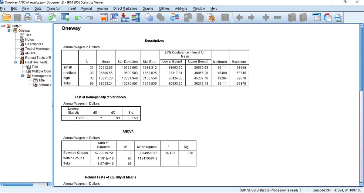
The Viewer shows a Oneway heading with Descriptives, Test of Homogeneity of Variances, ANOVA, Robust Tests of Equality of Means and Post Hoc Tests. In Descriptives, check that every group’s N equals the employees you expect to see.
Watch: A missing wage or responsibility code removes that employee from every table without a warning. If the group Ns fall short of the employees in the file, find out why before reading the F test.
Check the Test of Homogeneity of Variances
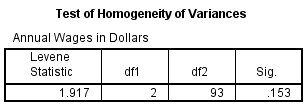
The Levene table gives the statistic, df1, df2 and Sig. It is shown for information, and it does not decide which result is reported.
Watch: A significant Levene test is not a reason to switch tables after the fact. Judge the SDs and group sizes in Descriptives as well.
Read the ANOVA and Robust Tests Tables
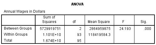
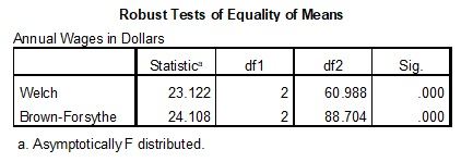
The ANOVA table gives the classical F with its two df, and Robust Tests of Equality of Means gives the Welch and Brown-Forsythe statistics with fractional df. Read the Welch row as the result when it is the default you chose.
Tip: The ANOVA table prints sums of squares, so eta squared can be computed as the between-groups sum of squares divided by the total. The Welch table prints no effect size.
Read the Multiple Comparisons Table
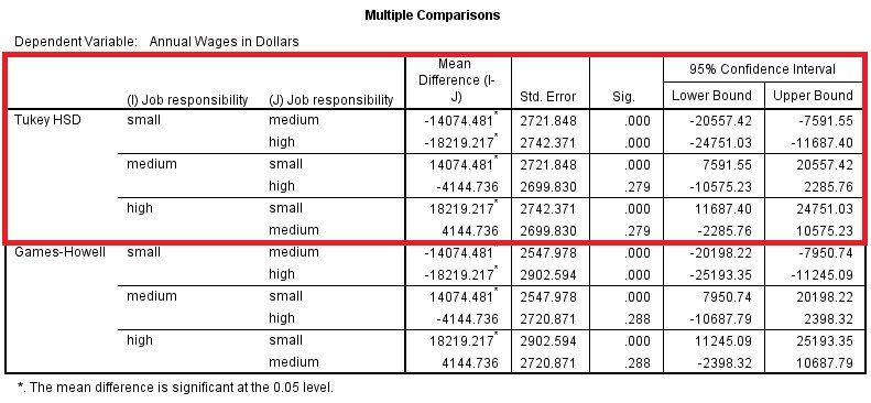
The Multiple Comparisons table lists Tukey HSD rows and Games-Howell rows, each pair in both directions. The red rectangle in the video screenshot marks the Tukey rows. Read the Mean Difference (I-J), the Sig. and the 95% confidence interval.
Watch: Each comparison appears twice with the sign reversed, and the asterisk only marks significance at .05. Report the mean difference and its interval, not the asterisk.
READING THE OUTPUT
Reading Descriptives, ANOVA, Robust Tests and Post Hoc
The table picks out SPSS output values for this one-way ANOVA, one per row, each with its video figure and a note on reading it in your data.
| Output value | In the example | How to read it |
|---|---|---|
| N and df | 31, 33 and 32 (total 96) | Valid cases per group. The within-groups df of 93 is 96 cases minus 3 groups |
| Mean and Std. Deviation | Small 22612.06 (10792.06), Medium 36686.55 (9500.50), High 40831.28 (12221.95) | Mean wage and its spread per group, in dollars. The SD column, not Std. Error, is the one to report |
| Levene Statistic and Sig. | 1.917 and .153, df 2 and 93 | Read beside the SDs, which range from 9,500 to 12,222 dollars, a largest-to-smallest ratio near 1.3 |
| ANOVA F, df and Sig. | 24.193, 2 and 93, .000 | The classical test. Sig. .000 is read as p < .001, and it does not say which groups differ |
| Sums of Squares | Between 5729919751, Total 1.674E+10 | Eta squared is between over total, 5729919751 / 1.674E+10, about .34 |
| Welch and Brown-Forsythe | 23.122 (df 2 and 60.988) and 24.108 (df 2 and 88.704), both .000 | The robust tests have fractional df. Both print, and one is reported |
| Tukey HSD Mean Difference | Small vs medium -14074.481, small vs high -18219.217, medium vs high -4144.736 | Mean Difference (I-J) in dollars. Only the medium vs high row, Sig. .279, has an interval containing zero |
| Games-Howell Sig. | .000, .000 and .288 | Same pattern with unequal variances allowed. Its standard errors and intervals differ somewhat from Tukey’s, pair by pair |
COMMON MISTAKES
Slips to Avoid With the F Test and Post Hoc Pairs
Six mistakes follow, each tied to a stage (data setup, SPSS dialogs, output or write-up) and each paired with a brief note on how to avoid it.
A Significant F Read as Every Group Different The F test says only that not all population means are equal. Here the medium vs high difference is not statistically significant (Sig. .279 and .288), and only the post hoc rows show which pairs differ.
Welch and Post Hoc Ticks Lost Without Syntax The Options and Post Hoc ticks are easy to lose between sessions. Pasting the command instead of clicking OK keeps the Welch and Games-Howell settings in a syntax file, so the run can be repeated and checked.
Causal Wording for an Observed Grouping Job responsibility is recorded, not assigned. The result describes differences in wage between groups, and wording such as the effect of responsibility on wage claims more than the design supports.
Post Hoc Family Not Named in the Report Tukey and Games-Howell rows print together, and their intervals differ slightly for the same pair. A write-up that quotes one pair from each block mixes methods, so it names the family it reports.
A Skewed Group Left Unplotted The small group has a long right tail, with wages up to 58,999 against a mean near 22,600. Plot each group and, when the shape is a concern, repeat the comparison with a rank-based test.
Stopping at the p-Value A significant F says nothing about size. Report an effect size such as eta squared, the group means with their SDs, and the mean differences with their intervals.
If you have already run this test, Independent Statistical Review has an OnlineSPSS statistician check the table, the post hocs and eta squared against your output.
SOURCES
Sources and Further Reading
Each source listed here backs a statement on this page, and the line beneath it tells you what to read it for.
Delacre, M., Leys, C., Mora, Y. L., & Lakens, D. (2019). Taking parametric assumptions seriously: Arguments for the use of Welch's F-test instead of the classical F-test in one-way ANOVA. International Review of Social Psychology, 32(1), Article 13. DOI: 10.5334/irsp.198
Read this for the case for reporting the Welch test by default.
Lumley, T., Diehr, P., Emerson, S., & Chen, L. (2002). The importance of the normality assumption in large public health data sets. Annual Review of Public Health, 23(1), 151-169. DOI: 10.1146/annurev.publhealth.23.100901.140546
Read this for when a test of means holds up with skewed data.
Lakens, D. (2013). Calculating and reporting effect sizes to facilitate cumulative science: A practical primer for t-tests and ANOVAs. Frontiers in Psychology, 4, Article 863. DOI: 10.3389/fpsyg.2013.00863
Read this for how eta squared and omega squared are defined.
FREQUENTLY ASKED QUESTIONS
Menus, Group Shape and Post Hoc Tests in the Example
Four questions are answered here. They deal with the SPSS screens, the method behind this analysis, the example in the video and how to report what it shows.
Why does the One-Way ANOVA dialog look different in my SPSS?
The video was recorded in an older release of IBM SPSS Statistics. Recent releases rename the submenu Compare Means and Proportions. This page makes no claim about other changes in the dialog, and its eta squared and omega squared come from the printed sums of squares, so no figure below depends on a release option.
Must wages be normally distributed within each group?
The assumption refers to each group’s own distribution, and moderate departures are usually tolerated when groups are reasonably large (Lumley et al., 2002). Strong skew in small groups can leave even the Welch test short of its nominal error rate, and a rank-based or trimmed-means comparison is advised as a cross-check (Delacre et al., 2019).
Tukey or Games-Howell for the follow-up comparisons?
Tukey assumes equal variances and Games-Howell does not, so Games-Howell fits the Welch default. Here both agree: small differs from medium (-14,074.48 dollars, 95% CI [-20,198.22, -7,950.74]) and from high (-18,219.22, 95% CI [-25,193.35, -11,245.09]) with Games-Howell, while medium vs high is not statistically significant (p = .288, 95% CI [-10,687.79, 2,398.32]).
How is a Welch F(2, 60.99) of 23.12 written up?
With the group summaries, the test and an effect size, then the Games-Howell pairs above. Small (M = 22,612.06, SD = 10,792.06, n = 31), medium (M = 36,686.55, SD = 9,500.50, n = 33) and high (M = 40,831.28, SD = 12,221.95, n = 32): Welch F(2, 60.99) = 23.12, p < .001, with eta squared = .34 and omega squared = .33 from the ANOVA table (Lakens, 2013).
NEXT STEP
Need a Three-Group Mean Comparison
Run or Checked?
OnlineSPSS is a statistical consultancy for researchers. Share your design and dataset, and a statistically trained Research Coordinator reviews it. The scope and one fixed project fee are confirmed before work begins.
No Commitment Required
Strictly Confidential
Fixed Project Fee
In-House PhD-Level Statisticians
Same-Day Response
Serving Researchers Since 2014