
One-Sample t-Test in SPSS
Video Walkthrough of a Worked Benchmark Example
This one-sample t-test in SPSS video sets the mean of 37 math test scores against a fixed value of 86 in the One-Sample T Test dialog. The page adds where a test value comes from, how the two tables are read and what Cohen's d adds beside the p-value.
WATCH THE VIDEO
One-Sample t-Test in SPSS, Start to Finish
Fix the test value, and note where it came from, before the sample is examined: the test asks whether the population mean differs from that value, not whether the sample resembles a population. Read the result as a mean difference with its 95% interval. In this example the sample mean lies 12.92 points below 86 and the interval excludes zero.
IN SHORT
What the Video Shows in Brief
In this one-sample t-test in SPSS video, the mean of a math test score (n = 37) is compared with a test value of 86. The path is Analyze, Compare Means, One-Sample T Test, with the score in Test Variable(s) and 86 in Test Value. The sample mean is 73.08 (SD = 16.90) and the mean difference is -12.92 points, 95% CI [-18.55, -7.29], t(36) = -4.65, p < .001: statistically significant, and the interval excludes zero.
BEFORE YOU RUN
What a Benchmark Test Needs From Your Data
Each of the four points below is a check on the study design or the data, made before any output is produced in SPSS.
A Value From Outside the Data The test value is a benchmark, norm or target fixed before the data are seen. The video treats 86 as the population mean without giving its source, which a write-up would name.
One Measurement per Case Each case contributes one independent score. Pre and post scores from the same participant make the question a paired one, and participants drawn from a few classrooms need a model that allows for the clustering.
An Outcome With Meaningful Differences A mean needs equal steps on the scale, as with a test score from 1 to 100. An ordinal outcome, such as a short agreement rating, points to a test on the median or on ranks instead.
The Scores Within the Sample The test concerns the mean, so look at a histogram first. A t-test of a mean holds up under moderate skew in moderately large samples (Lumley et al., 2002), while strong skew, outliers or a very small sample need more care.
STEP BY STEP
Running the One-Sample T Test Dialog
Screenshots of IBM SPSS show what you will see along the way. The numbered steps below give the menu path and the settings, each with a check or a tip.
Each slide pairs with one step through its number and shows the SPSS screen at that point. Newer releases may word some labels slightly differently from the older one used in the video.


Open the One-Sample T Test Dialog
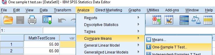
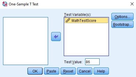
Choose Analyze, then Compare Means (Compare Means and Proportions in recent releases), then One-Sample T Test. The dialog that opens lists the variables at left, with a Test Variable(s) box and a Test Value box.
Check: The comparison here is with a number typed into the dialog. If the benchmark exists as data, such as the scores of a second group in the file, a two-sample test fits instead.
Set the Variable and the Test Value
Move the score (MathTestScore, labeled Test results (1 to 100)) into the Test Variable(s) box, type 86 in the Test Value box and select OK.
Tip: Bootstrap, beside Options, adds a bootstrap confidence interval for the mean difference, a cross-check that leans less on the shape of the scores where that module is licensed.
Check the Command in the Log
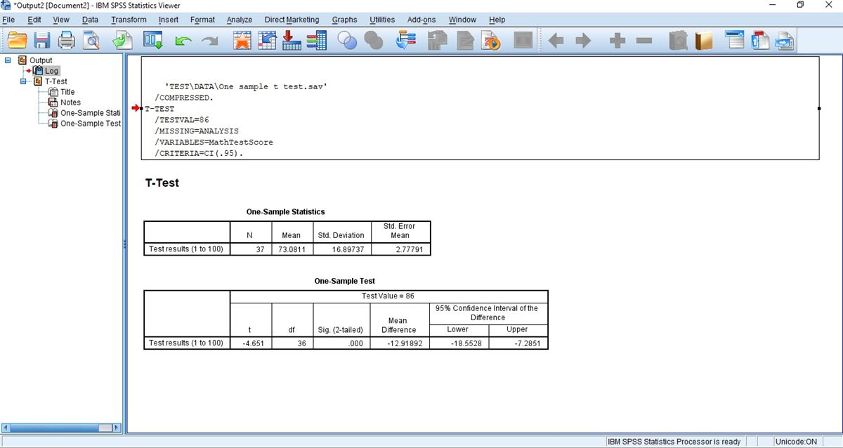
The Viewer opens with the T-TEST command in the Log: TESTVAL=86, MISSING=ANALYSIS, the variable name and CRITERIA=CI(.95). Compare TESTVAL with the value you intended before reading any result.
Tip: CRITERIA=CI(.95) sets the 95% level of the interval in the Test table. A different level under Options changes the interval limits but not t, df or Sig.
Read the One-Sample Statistics
The first table gives N, Mean, Std. Deviation and Std. Error Mean of the score. Confirm that N matches the number of cases you expect before reading the test itself.
Check: The table prints four or five decimals. Round from these figures, so that an SD of 16.89737 becomes 16.90 and not 16.89.
Read the One-Sample Test
The second table repeats the Test Value in its header and lists t, df, Sig. (2-tailed), Mean Difference and the 95% confidence interval of the difference. Read the interval with the mean difference, not the p-value alone.
Watch: The Mean Difference is the sample mean minus the test value, so -12.91892 means the sample mean lies below 86. The interval is for that difference, not for the mean itself.
READING THE OUTPUT
Reading One-Sample Statistics and the Test Table
For each value it lists from the SPSS output, the table gives the example figure from the video and explains how to read it in your own data.
| Output value | In the example | How to read it |
|---|---|---|
| N | 37 | Cases with a score. Compare it with the cases in the file. Degrees of freedom are N minus 1, which gives 36 here |
| Mean | 73.0811 | The sample mean of Test results (1 to 100), in points of the scale |
| Std. Deviation | 16.89737 | The spread of the scores around their mean, in the same points of the scale |
| Std. Error Mean | 2.77791 | The SD divided by the square root of N. It describes the precision of the mean, not the spread |
| t and df | -4.651 and 36 | The mean difference divided by its standard error. A negative t means the sample mean is below 86 |
| Sig. (2-tailed) | .000 | Two-sided p, read as p < .001. It shows that a difference is detectable, not how large it is |
| Mean Difference | -12.91892 | The sample mean minus the test value, 73.0811 minus 86, in points of the scale |
| 95% CI of the Difference | -18.5528 to -7.2851 | The differences between the population mean and 86 that are compatible with the data. Add 86 to each limit for an interval around the mean |
COMMON MISTAKES
Slips to Avoid With a Test Value
Some mistakes start in the data setup, others in the SPSS dialogs, the output or the write-up. Six of them follow, each with a short note on avoiding it.
Reading .000 as Zero SPSS prints .000 when the p-value rounds to zero at three decimals. It means p < .001, and a write-up that says p = .000 states a probability of exactly zero.
One Test Value for Several Variables The Test Value box applies to every variable in the Test Variable(s) list. Scores on different scales, each with its own benchmark, need separate runs, and the number of tests is reported.
Missing Scores Dropped Without a Message The command shows MISSING=ANALYSIS, so cases without a score leave the test silently. The N in One-Sample Statistics is the first place it shows, so compare it with the number of cases in the file.
A Histogram Never Requested The One-Sample T Test dialog draws no plot, and the video shows none. The 37 scores run from 45 to 100 with a gap between 69 and 81, which a histogram would show and the tables do not.
TESTVAL=86 With No Recorded Source The Log records TESTVAL=86 but not where 86 came from. Paste the command, name the source in a syntax comment and again in the write-up, so a reader can judge whether the comparison is fair.
Stopping at Significant A significant result says the mean differs from 86 and nothing about how far. Report the mean difference, here -12.92 points, with its interval, and a standardized effect size if the field expects one.
If you have already run this test, Independent Statistical Review has an OnlineSPSS statistician check the test value, the interval and the wording in your output.
SOURCES
Sources and Further Reading
Statements on this page draw on the literature listed below, and a line under each entry says what it is worth reading for.
Lumley, T., Diehr, P., Emerson, S., & Chen, L. (2002). The importance of the normality assumption in large public health data sets. Annual Review of Public Health, 23(1), 151-169. DOI: 10.1146/annurev.publhealth.23.100901.140546
Read this for when a t-test of a mean holds up with skewed data.
Lakens, D. (2013). Calculating and reporting effect sizes to facilitate cumulative science: A practical primer for t-tests and ANOVAs. Frontiers in Psychology, 4, Article 863. DOI: 10.3389/fpsyg.2013.00863
Read this for how Cohen's d is built from a mean difference and an SD.
FREQUENTLY ASKED QUESTIONS
Menus, Shape and Effect Size in the Example
From the SPSS menus on your screen to the final write-up, the questions here follow this analysis, taking in the method and the video example.
Why does the One-Sample T Test dialog look different in my SPSS?
The video was recorded in an older release of IBM SPSS Statistics. From release 27 the dialog has an Estimate effect sizes option that prints a One-Sample Effect Sizes table, and recent releases name the submenu Compare Means and Proportions. The Test Variable(s) box, the Test Value box and both main tables sit as shown in the video.
Do the scores in the example suit a t-test?
The video shows no histogram, but the data file holds 37 scores with a flat shape, skewness near 0.08 and no outliers. A test of the mean depends on the sampling distribution of the mean, which nears normality fastest for symmetric data without outliers (Lumley et al., 2002), so the shape is a minor concern here.
How large is the gap in standard deviation units?
Cohen’s d is (73.0811 minus 86) divided by 16.89737 = -0.76, with the sample SD as the standardizer, the same form as the dz of a paired design (Lakens, 2013). The video’s release prints no effect size, so d is computed from the printed mean difference and SD, and the write-up names the standardizer used.
How is a gap of 12.92 points below 86 written up?
With the sample mean and SD, the value it was tested against, the difference with its 95% interval, and Cohen’s d. Math test score (M = 73.08, SD = 16.90, n = 37) against a test value of 86: mean difference -12.92, 95% CI [-18.55, -7.29], t(36) = -4.65, p < .001, Cohen’s d = -0.76. A real write-up names the source of 86 beside it, which the video does not give.
NEXT STEP
Need a Benchmark Comparison
Run or Checked?
OnlineSPSS is a statistical consultancy for researchers. Share your design and dataset, and a statistically trained Research Coordinator reviews it. The scope and one fixed project fee are confirmed before work begins.
No Commitment Required
Strictly Confidential
Fixed Project Fee
In-House PhD-Level Statisticians
Same-Day Response
Serving Researchers Since 2014