
Kaplan-Meier Survival Analysis in SPSS
Video Walkthrough With a Log-Rank Test
This Kaplan-Meier survival analysis in SPSS video compares weeks to relapse between a detox group and a treatment group with a log-rank test. The page adds how censoring is coded, why the mean is limited and what a non-significant log-rank result leaves open.
WATCH THE VIDEO
Kaplan-Meier Survival Analysis in SPSS, Start to Finish
Report the median survival time with its interval beside the log-rank result, and state how many cases were censored. Here the medians are 9 weeks for detox and 17 for treatment, but the treatment interval runs from 0 to 35.7 weeks, past the 30 weeks of follow-up, and the log-rank test gives p = .112. That is not statistically significant, which differs from showing that survival is alike.
IN SHORT
What the Video Shows in Brief
In this Kaplan-Meier survival analysis in SPSS video, weeks to relapse are compared between a detox group and a treatment group of 20 cases each, with Event coded 1 and censored cases 0. The path is Analyze, Survival, Kaplan-Meier. There are 17 and 13 events, and the Log Rank (Mantel-Cox) test gives chi-square(1) = 2.528, p = .112: not statistically significant.
BEFORE YOU RUN
Checks on Time, Status and Censoring Before Kaplan-Meier
These four points cover what to check in your study design and data, and each one is settled before the analysis is run in SPSS.
An Event and a Time Origin Each case needs a time and a status: weeks to the event, coded 1, or weeks to the end of follow-up, coded 0. Time must start at the same point in both groups and run in one unit, here weeks to relapse.
Censoring Unrelated to the Outcome Censored cases are assumed as likely to have the event later as those still followed (Clark et al., 2003). Here 3 of 20 detox and 7 of 20 treatment cases are censored, six of the seven at week 30 and one at week 19.
Two Separate Groups Group is a factor with detox coded 0 and treatment coded 1, and no case appears in both. Without random allocation, the groups can differ in other ways, and adjusting for them is a job for Cox regression.
Curves That Do Not Cross The log-rank test weights all time points equally and suits curves that stay apart in one direction. Crossing curves can cancel in the single statistic, so check the curves in your own output before trusting it.
STEP BY STEP
Setting Up Time, Status and Factor in Kaplan-Meier
The screenshots show each screen in IBM SPSS, and the numbered steps below give the menu path, the settings to choose and a check or tip for each step.
Numbered by step, the slides hold the SPSS screen one step at a time. Your release may label a few items differently, since the video was recorded in an older one.
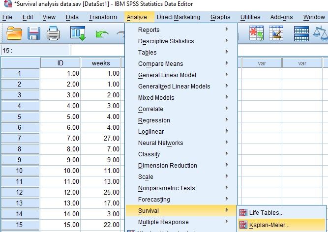
Open the Kaplan-Meier Dialog
Choose Analyze, then Survival, then Kaplan-Meier. In the screenshot, ID and weeks are the first two columns of the Data Editor.
Check: The Survival submenu also lists Life Tables, which group time into intervals. One time in weeks per case belongs in Kaplan-Meier.
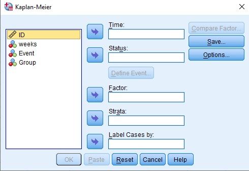
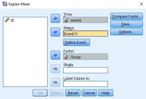
Move Weeks, Event and Group Into the Boxes
Move weeks into Time, Event into Status and Group into Factor. Status reads Event(?) until its event value is defined, and ID, Strata and Label Cases by stay unused.
Watch: Compare Factor stays grayed out until a Factor variable is entered. Strata, left empty here, would run the comparison within layers of another variable.
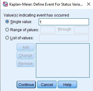
Set Single Value 1 in Define Event
Select Define Event, keep Single value and enter 1, the code for the event, then select Continue. Range of values and List of values stay empty.
Check: The value entered is the code for the event, not for survival. Entering 0 would treat the censored cases as events and the real events as censored.
Tick Log Rank Under Compare Factor
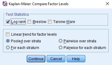
Select Compare Factor, tick Log rank under Test Statistics and keep Pooled over strata, then select Continue. Breslow and Tarone-Ware stay unticked.
Tip: Breslow and Tarone-Ware weight early times more than Log rank does. Name the test in the analysis plan, because choosing among them after the results can steer the p-value.
Tick Survival Table and Mean and Median
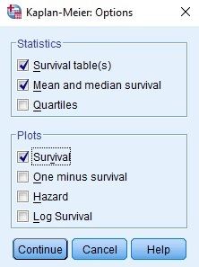
Select Options and tick Survival table(s) and Mean and median survival under Statistics, and Survival under Plots. Quartiles stays unticked. Then select Continue and OK.
Check: Quartiles, unticked here, would add the 25th and 75th percentiles of survival time. A percentile exists only if the curve falls that far, which heavy censoring can prevent.
Read the Case Processing Summary
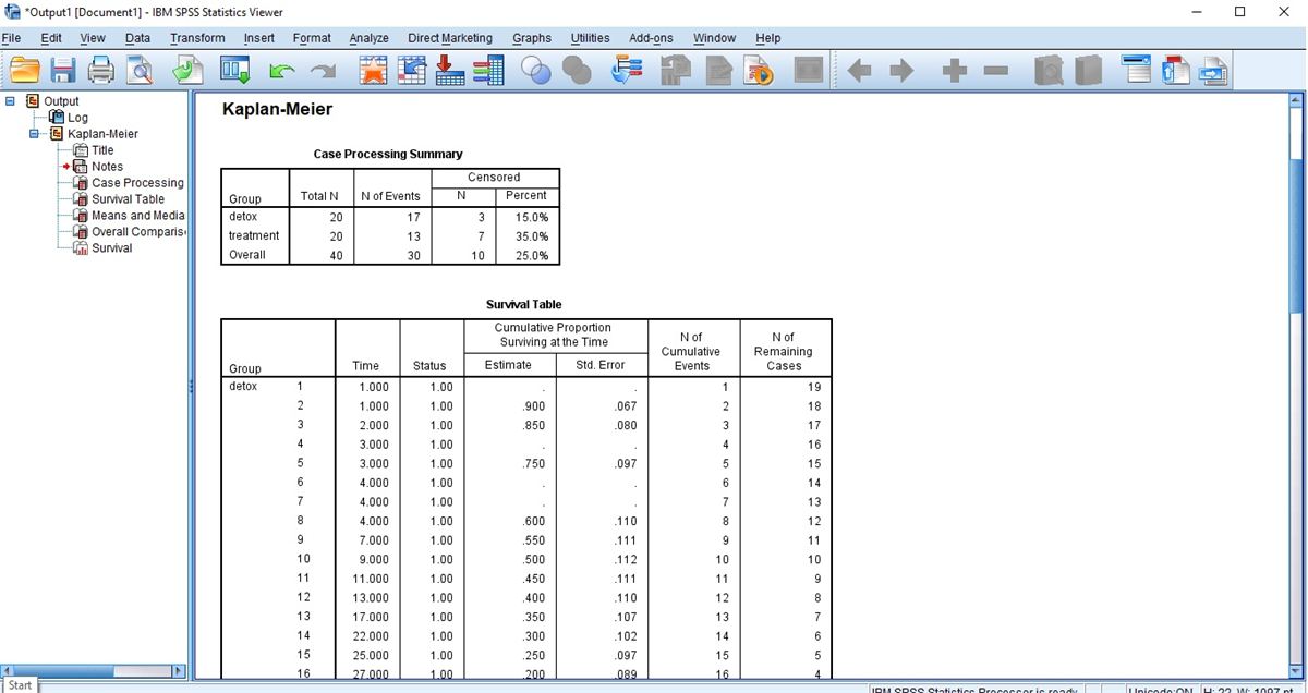
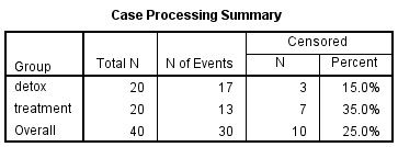
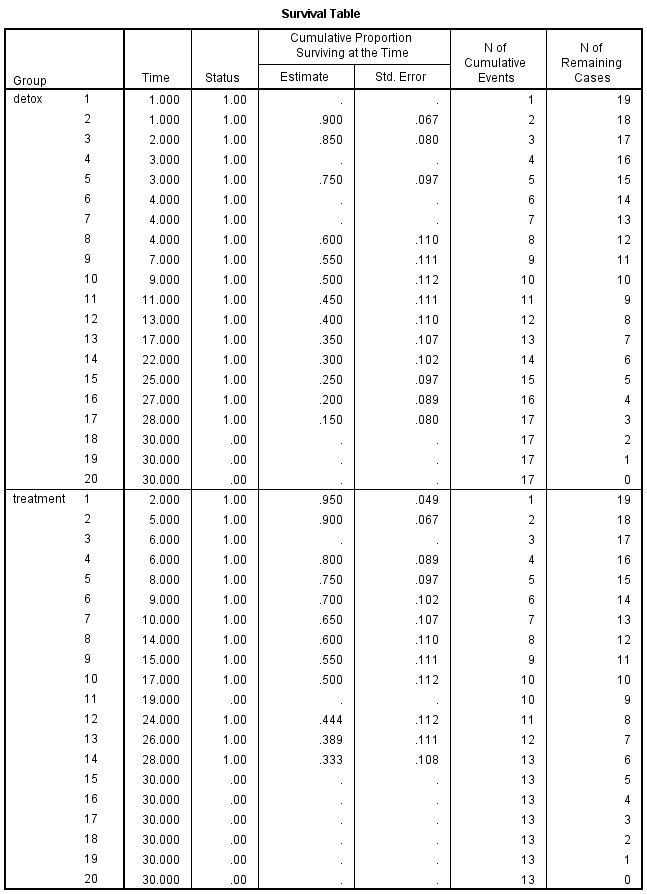
The Viewer opens with Case Processing Summary, then Survival Table, Means and Medians for Survival Time and Overall Comparisons. Detox has 20 cases, 17 events and 3 censored (15.0%), and treatment has 20, 13 and 7 (35.0%).
Watch: The Survival Table prints an estimate only on the last of the cases tied at one time, so time 1.000 shows a dot and then .900. The dots are not missing data, and censored rows carry dots too.
Read Means, Medians and Log Rank
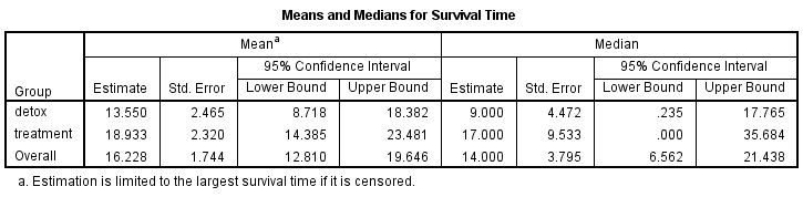
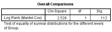
Means and Medians for Survival Time gives medians of 9.000 weeks for detox and 17.000 for treatment, with 95% intervals. Overall Comparisons gives Log Rank (Mantel-Cox) Chi-Square 2.528, df 1 and Sig. .112.
Tip: Write the statistic as chi-square(1) = 2.528, p = .112. SPSS labels the column Chi-Square, and its Sig. belongs to the Log Rank (Mantel-Cox) row.
READING THE OUTPUT
Reading Medians, Means and Log Rank (Mantel-Cox)
Each row of the table names one value in the SPSS output, gives its figure in the video example and says how to read it for your own data.
| Output value | In the example | How to read it |
|---|---|---|
| Case Processing Summary | Detox 20, 17 events, 3 censored; treatment 20, 13, 7 | Events and censored cases per group. A censored case was still event-free when follow-up ended |
| Survival Table, Estimate | Detox .900 at week 1 to .150 at week 28; treatment .950 at week 2 to .333 at week 28 | The cumulative proportion still event-free. Dots mark tied times and censored rows |
| Mean, Estimate | Detox 13.550, treatment 18.933 | The restricted mean: the area under the curve up to 30 weeks, the largest time, which is censored (table footnote) |
| Median, Estimate | Detox 9.000, treatment 17.000 | The first time the curve reaches .500, which is the usual summary under censoring |
| Median, 95% CI | Detox .235 to 17.765, treatment .000 to 35.684 | The normal-approximation interval SPSS prints for each median |
| Log Rank (Mantel-Cox) | Chi-Square 2.528, df 1, Sig. .112 | Tests whether the two survival distributions are equal; Sig. is its p-value |
| Survival plot | Requested, not pictured | Ticked under Plots in Options; no curve image is used on this page, so nothing is read from it |
COMMON MISTAKES
Slips With Censored Rows, the Mean and Hazard Ratios
Six mistakes with this survival analysis are set out below. Each comes from the data setup, dialogs, output or write-up, with a short note on avoiding it.
Censored Cases Dropped From the Data A case lost to follow-up stays in the file with Status 0 and its last observed week. Deleting such cases, or coding them as events, shortens follow-up and biases the survival estimates downward.
Mean Survival Quoted as the Summary Estimation is limited to the largest survival time when it is censored, and here that is 30 weeks in both groups, so 13.550 and 18.933 understate the means. Quote the medians with their intervals.
Direction Read From the Chi-Square Chi-square 2.528 has no sign. Computed outside SPSS, equal survival would give about 12.8 detox and 17.2 treatment events against 17 and 13 observed, so detox had more events than expected (Bland & Altman, 2004).
A Hazard Ratio Expected From Log Rank Overall Comparisons gives a chi-square and a Sig. and nothing about size (Bland & Altman, 2004). A hazard ratio with its interval needs Cox regression, which this video does not cover.
Days and Weeks in One Time Column A time column that mixes days and weeks gives medians in no unit at all. Keep one unit, name it in the variable label, weeks here, and repeat it in the report.
Second Relapses Entered as New Rows Kaplan-Meier models time to the first event. A person who relapses twice and fills two rows enters as two independent cases, which understates the uncertainty. Keep one row per person.
If you have already run this test, Independent Statistical Review has an OnlineSPSS statistician check the censoring, the medians and the wording against your output.
SOURCES
Sources and Further Reading
The sources below support statements made on this page, and the line under each entry says what to read it for.
Clark, T. G., Bradburn, M. J., Love, S. B., & Altman, D. G. (2003). Survival analysis part I: Basic concepts and first analyses. British Journal of Cancer, 89(2), 232-238. DOI: 10.1038/sj.bjc.6601118
Read this for censoring and the Kaplan-Meier estimate explained plainly.
Bland, J. M., & Altman, D. G. (2004). The logrank test. BMJ, 328(7447), 1073. DOI: 10.1136/bmj.328.7447.1073
Read this for the logic of comparing observed with expected events.
FREQUENTLY ASKED QUESTIONS
Menus, Median Limits and Table Steps in the Example
Each question below concerns this analysis in SPSS: why a screen may differ from the video, a point of method, a figure in the example or the write-up.
Why does the Kaplan-Meier dialog look different in my SPSS?
The video was recorded in an older release of IBM SPSS Statistics. IBM’s release 23 page for Compare Factor Levels lists Log rank, Breslow and Tarone-Ware, says Log rank weights all time points equally, and describes Pooled over strata as one test of all factor levels. The video’s dialog shows the same three tests.
Why does the treatment median interval start at .000?
SPSS builds the interval as the median plus or minus 1.96 standard errors: 17 plus or minus 1.96 x 9.533 gives -1.68 to 35.68. A survival time cannot be negative, so the table shows .000, and the upper limit lies beyond the 30 weeks observed. The interval says the median is poorly determined.
How does the detox curve reach .500 at week 9?
At each event time the estimate is multiplied by the share of cases still followed that stay event-free. Detox goes from 2 of 20 in week 1 to .900, 1 of 18 in week 2 to .850, 2 of 17 in week 3 and 3 of 15 in week 4 to .600, 1 of 12 in week 7 to .550 and 1 of 11 in week 9 to .500.
How are chi-square(1) = 2.528 and the two medians written up?
Name the method, the events and medians per group, and the test. Kaplan-Meier estimates were compared with a log-rank test. Median time to relapse was 9.00 weeks for detox (n = 20, 17 events, 95% CI [0.24, 17.77]) and 17.00 for treatment (n = 20, 13 events, [0.00, 35.68]); the difference was not statistically significant, chi-square(1) = 2.528, p = .112.
NEXT STEP
Need a Time-to-Event Comparison
Run or Checked?
OnlineSPSS is a statistical consultancy for researchers. Share your design and dataset, and a statistically trained Research Coordinator reviews it. The scope and one fixed project fee are confirmed before work begins.
No Commitment Required
Strictly Confidential
Fixed Project Fee
In-House PhD-Level Statisticians
Same-Day Response
Serving Researchers Since 2014