
One-Way MANOVA in SPSS
Video Walkthrough of a Worked Test Score Example
This one-way MANOVA in SPSS video asks whether male and female participants differ on English, Math and History scores taken together. The page adds the choice among the four multivariate statistics, what Box's M and Levene check, and the follow-up tests.
WATCH THE VIDEO
One-Way MANOVA in SPSS, Start to Finish
Name the multivariate statistic you will report before the output is opened. With two groups, as here, the factor has a single dimension, so Pillai’s trace, Wilks’ lambda, Hotelling’s trace and Roy’s largest root print the same F and p and the choice changes nothing. With three or more groups they can disagree, and in simulations of six MANOVA tests Pillai’s trace was the most robust when assumptions failed (Olson, 1974).
IN SHORT
What the Video Shows in Brief
In this one-way MANOVA in SPSS video, English, Math and History scores are compared between 42 male and 35 female participants. The path is Analyze, General Linear Model, Multivariate, with the three scores as Dependent Variables and Gender as Fixed Factor. Wilks’ lambda is .983, F(3, 73) = 0.42, p = .740, partial eta squared = .017: not statistically significant.
BEFORE YOU RUN
Checks on Scores and Covariances Before Multivariate
The four points below concern your study design and your data. Settle each one first, then run this one-way MANOVA in SPSS.
Independent Cases Every participant belongs to a single gender group and gives one row, which the design settles. Repeated testing of the same people needs a repeated measures model, and participants nested in classes need a multilevel model.
Outcomes That Belong Together The three scores are one set. Where each outcome is a question of its own, separate ANOVAs can serve without a preliminary MANOVA (Huberty & Morris, 1989). Each group also needs more cases than outcomes, here 42 and 35 against 3.
Shape and Outliers Within Groups MANOVA assumes multivariate normal scores within each group, which no single test settles. Inspect each score by gender and screen for multivariate outliers, for example with Mahalanobis distance.
Covariance Matrices Equal covariance matrices of the three scores matter most when group sizes differ, as 42 and 35 do. Judge them from the matrices and the sample sizes, with Box's M as one input and not as a gate.
STEP BY STEP
Setting Up the Multivariate Dialog, Model and Options
Follow the numbered steps below through IBM SPSS, with screenshots as you go: each step gives the menu path, the settings to pick and a check or tip.
Each numbered slide captures what SPSS displays at one step of this one-way MANOVA. The recording comes from an older release, so a few labels may not match your version.
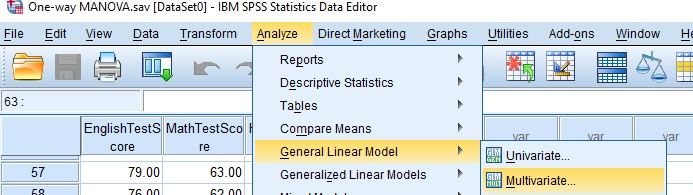
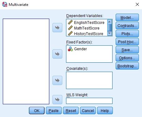
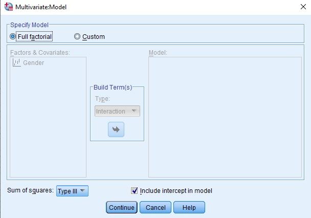
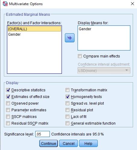
Open the Multivariate Dialog
Choose Analyze, then General Linear Model, then Multivariate. The dialog opens with Dependent Variables, Fixed Factor(s), Covariate(s) and WLS Weight boxes, and buttons for Model, Contrasts, Plots, Post Hoc, Save, Options and Bootstrap.
Check: Several outcomes analyzed together belong in Multivariate. One outcome belongs in Univariate, and the same people measured repeatedly belong in Repeated Measures.
Fill Dependent Variables and Fixed Factor(s)
Move EnglishTestScore, MathTestScore and HistoryTestScore into Dependent Variables and Gender into Fixed Factor(s). In Model, Full factorial with Type III sum of squares and the intercept included is already selected and suits one factor.
Watch: Enter only outcomes that the research question names. Each score added raises the number of cases every group needs and adds one more follow-up test to the family.
Tick Effect Size and Homogeneity Tests
In Options, move Gender into Display Means for. Under Display, select Descriptive statistics, Estimates of effect size and Homogeneity tests. The significance level stays .05, then select Continue and OK.
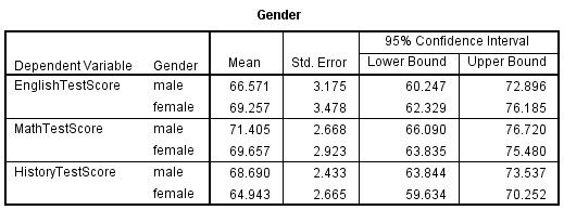
Tip: Display Means for Gender produces the Estimated Marginal Means table at the end of the output. With a single factor its means equal the observed means, so it adds more once a second factor is in the model.
Check Group Sizes Under General Linear Model
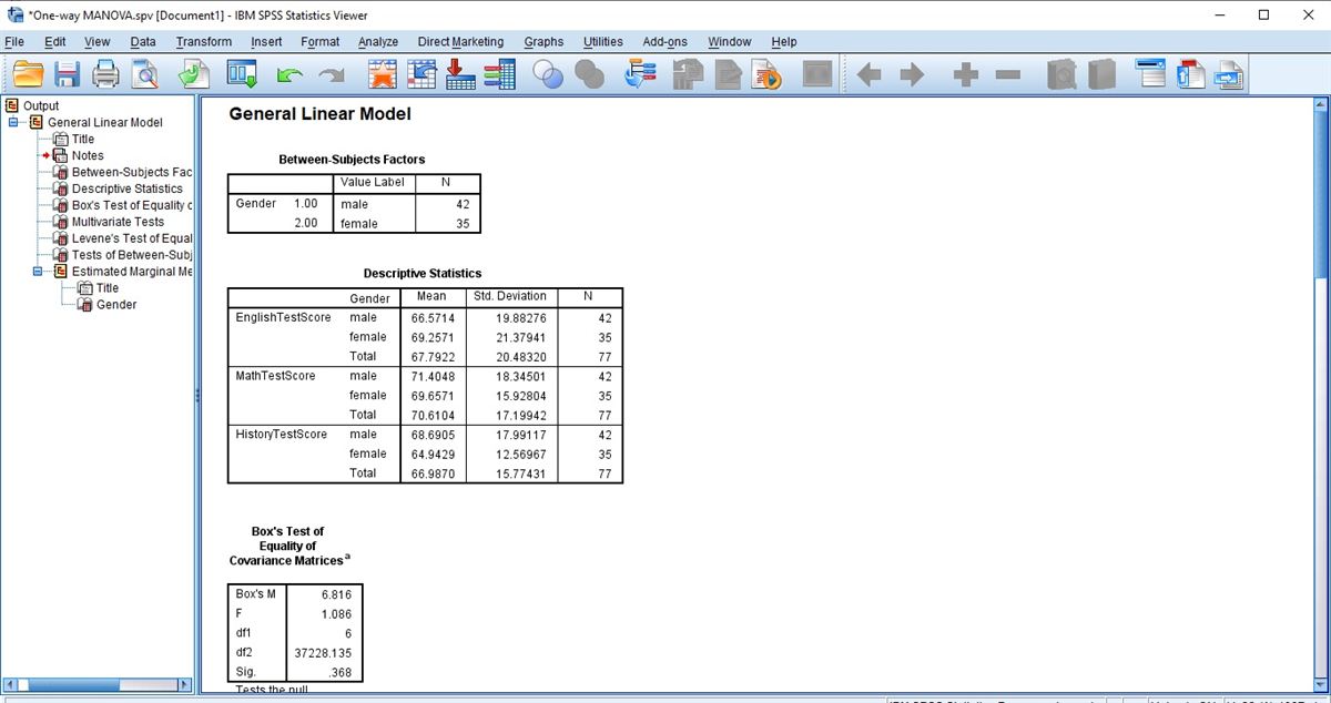
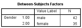
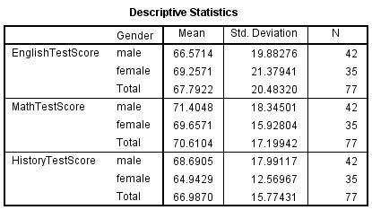
The Viewer opens with the General Linear Model heading, then Between-Subjects Factors (Gender 1 male, N = 42; 2 female, N = 35) and Descriptive Statistics with the mean, Std. Deviation and N of each score by gender and in total.
Watch: A case missing any one of the three scores drops out of the whole analysis. The N of 77 here should equal the number of rows that have all three scores.
Read Box's M Before the Multivariate Tests
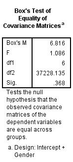
Box’s M is 6.816, F = 1.086 with df 6 and 37228.135, Sig. .368. It tests the null hypothesis that the population covariance matrices of the three scores are equal in the two gender groups.
Tip: Box’s M reacts to nonnormal scores as well as to unequal matrices. A large p gives no evidence against equal covariance matrices, though it cannot show that they are equal.
Read the Multivariate Tests Table
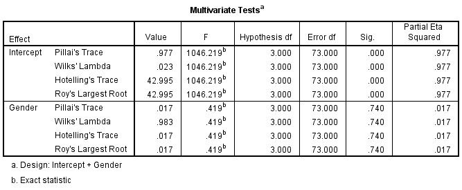
The Gender block has four rows, Pillai’s Trace, Wilks’ Lambda, Hotelling’s Trace and Roy’s Largest Root, each with Value, F, Hypothesis df 3, Error df 73, Sig. and Partial Eta Squared. The footnote on F reads Exact statistic.
Watch: Error df reads 73 here, while the Gender rows of the effects table use 75. The multivariate error df also allow for the three outcomes, so each test is quoted with its own pair of df.
Read Levene and Between-Subjects Effects
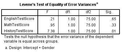
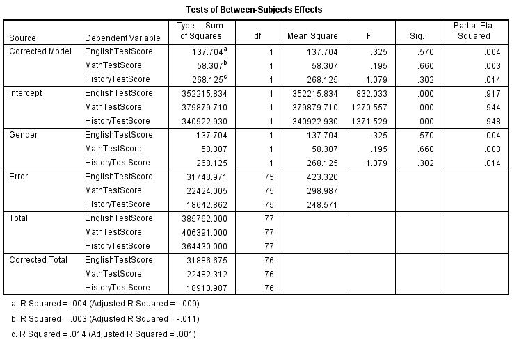
Levene’s Test of Equality of Error Variances gives one row per score. Tests of Between-Subjects Effects lists Corrected Model, Intercept, Gender, Error, Total and Corrected Total for each score, so read the Gender rows. Estimated Marginal Means closes the output.
Tip: The Corrected Model and Gender rows carry identical figures, because Gender is the only term in the model. With more terms they differ, and the row of the term of interest is the one to read.
READING THE OUTPUT
Reading Box's M, Wilks' Lambda and Gender Rows
Row by row, the table names a value in the SPSS output for this one-way MANOVA, its figure in the video example and how to read it in your data.
| Output value | In the example | How to read it |
|---|---|---|
| N | Male 42, female 35, total 77 | Cases per group. The error df of 75 is 77 cases minus 2 groups |
| Mean and Std. Deviation | English 66.57 (19.88) and 69.26 (21.38); Math 71.40 (18.35) and 69.66 (15.93); History 68.69 (17.99) and 64.94 (12.57) | Male and female scores in test points. Report the SD, not the standard error |
| Box’s M, F and Sig. | 6.816, 1.086 (df 6 and 37228.135), .368 | Covariance check shown for information, and a large p leaves equality unproven |
| Wilks’ Lambda, F and Sig. | .983, 0.419 (df 3 and 73), .740 | Lambda near 1 means little of the joint variance sits with Gender. The other three statistics repeat this F and p |
| Partial Eta Squared (multivariate) | .017 | Share of the joint variance linked to Gender in this sample, printed without an interval |
| Levene F and Sig. | English .21 (.65), Math .95 (.33), History 7.38 (.01), df 1 and 75 | One row per score. History has the smallest p and the widest gap in SDs |
| Gender row: F, Sig., partial eta squared | English .325, .570, .004; Math .195, .660, .003; History 1.079, .302, .014 | Three separate ANOVAs with df 1 and 75, each unadjusted for the three tests |
| Estimated Marginal Means | English male 66.571 (95% CI 60.247 to 72.896), female 69.257 (62.329 to 76.185) | Precision of each group mean in points. The table gives no interval for the gap between groups |
COMMON MISTAKES
Slips With Wilks' Lambda, Intercept Rows and Effect Sizes
Six mistakes with this one-way MANOVA are set out below. Each comes from the data setup, dialogs, output or write-up, with a short note on avoiding it.
Multivariate Eta Squared Quoted Per Score The .017 in Multivariate Tests describes the three scores as a set. Each score has its own value in the Gender rows, .004, .003 and .014, so a sentence giving .017 for History mixes the two levels.
Wilks' Lambda Without Its F and df A lambda of .983 cannot be judged alone. Report it with F, both df (3 and 73) and p, because the same lambda can be significant or not depending on the sample size and the number of outcomes.
Intercept Rows Read as the Result The Intercept rows show Sig. .000 and partial eta squared .977 in a model like this, because they test whether the grand means of the three scores are all zero. The group question sits in the Gender rows below them.
One Levene Row Prints Sig. .01 History has F = 7.38, with SDs of 17.99 for male and 12.57 for female participants. A detectable gap is not a verdict: judge its size against the group sizes of 42 and 35, and say that History was examined.
A Wilks' p Read as Equal Means A p of .740 gives no evidence against equal mean vectors and cannot show that the genders score alike. For English, the gap's 95% interval, computed outside SPSS, runs from about -12.1 to 6.7 points.
Gender Wording That Implies Cause Gender is a recorded attribute, so phrases like gender has an effect on English scores overstate what a group comparison shows. Write that scores were compared between male and female participants.
If you have already run this test, Independent Statistical Review has an OnlineSPSS statistician check the statistic, Box’s M and the follow-ups against your output.
SOURCES
Sources and Further Reading
The reading below supports what this page says about this one-way MANOVA, and a line under each entry notes what to read it for.
Olson, C. L. (1974). Comparative robustness of six tests in multivariate analysis of variance. Journal of the American Statistical Association, 69(348), 894-908. DOI: 10.1080/01621459.1974.10480224
Read this for how six MANOVA statistics fare when assumptions fail.
Huberty, C. J., & Morris, J. D. (1989). Multivariate analysis versus multiple univariate analyses. Psychological Bulletin, 105(2), 302-308. DOI: 10.1037/0033-2909.105.2.302
Read this for when separate ANOVAs can replace a preliminary MANOVA.
FREQUENTLY ASKED QUESTIONS
Menus, Multivariate Normality and Follow-Up Tests in the Example
Each question below concerns this analysis in SPSS: why a screen may differ from the video, a point of method, a figure in the example or the write-up.
Why does the Multivariate dialog look different in my SPSS?
The video was recorded in an older release of IBM SPSS Statistics. IBM’s release 23 page for GLM Multivariate Options lists the same Display choices as the video. Its Compare main effects item offers LSD (no adjustment), Bonferroni or Sidak for pairwise comparisons of the estimated marginal means, not for the three univariate F tests.
Must the scores be multivariate normal within each group?
MANOVA assumes it, and no single test proves it. With groups of 42 and 35, the test of mean vectors tolerates moderate skew better than it would with small groups, while one extreme case can still pull the group means. This output prints no multivariate normality test, so the judgment rests on the plots and the outlier screen set out under Before You Run.
Do the three univariate tests need an alpha adjustment?
Yes when each is read as its own finding. The Gender rows are unadjusted, so a Bonferroni level is .0167, one third of .05, and the p-values .570, .660 and .302 clear no such bar. Holm’s step-down method gives the same familywise protection and never less power. A preliminary MANOVA as the only protection has been challenged (Huberty & Morris, 1989).
How is a Wilks' lambda of .983 written up in APA 7?
Lead with the joint test, then the follow-ups. A one-way MANOVA on English, Math and History scores of male (n = 42) and female (n = 35) participants was not statistically significant, Wilks’ lambda = .983, F(3, 73) = 0.42, p = .740, partial eta squared = .017. Univariate p-values were .570, .660 and .302.
NEXT STEP
Need a Multi-Outcome Group Comparison
Run or Checked?
OnlineSPSS is a statistical consultancy for researchers. Share your design and dataset, and a statistically trained Research Coordinator reviews it. The scope and one fixed project fee are confirmed before work begins.
No Commitment Required
Strictly Confidential
Fixed Project Fee
In-House PhD-Level Statisticians
Same-Day Response
Serving Researchers Since 2014