
Two-Way ANOVA in SPSS
Video Walkthrough of a Worked Interaction Example
This two-way ANOVA in SPSS video asks whether happiness differs by gender and marital status among 94 people. The page adds why the interaction row comes first, what crossing lines in the plot do not show and how to word p = .669.
WATCH THE VIDEO
Two-Way ANOVA in SPSS, Start to Finish
Read the interaction row before any main effect, because a main effect is an average over the levels of the other factor (Maxwell et al., 2017). Here gender * maritalstatus gives F(4, 84) = 0.59, p = .669, which is no evidence that the gender gap varies with marital status. With cells of 8 to 13 people it is not proof of parallel lines, and the two main effects are read in that light.
IN SHORT
What the Video Shows in Brief
In this two-way ANOVA in SPSS video, happiness scores of 94 people are compared across gender (41 male, 53 female) and marital status (five groups of 17 to 22), with the interaction tested too. The path is Analyze, General Linear Model, Univariate, with happiness as Dependent Variable and both factors as Fixed Factor(s). The interaction gives F(4, 84) = 0.59, p = .669, partial eta squared .027: not statistically significant.
BEFORE YOU RUN
Checks on Ten Cells Before Fixed Factor(s)
Before you open the SPSS dialogs, the four points below need an answer from your study design and from the data themselves.
One Person in One Cell Each of the 94 people sits in exactly one gender by marital status cell, so observations are independent. Two ratings from one person, or people nested in households or clinics, need a repeated measures or multilevel model.
A Ten-Point Score as Continuous Happiness runs from 1 to 10 in the data, and an ANOVA treats the steps between scores as equal. That is a judgment about the scale, so state it in the write-up, and consider an ordinal model if the steps are doubtful.
Thin and Uneven Cells The ten cells hold 8 to 13 people, and their SDs run from 2.00 to 3.68. Normality and equal spread concern the errors within cells, so save the residuals and plot them, since a cell of 8 people shows little in any single test.
Two Recorded Factors, Fully Crossed Gender and marital status are recorded attributes, and every combination occurs. The interaction asks whether the gender difference changes with marital status, an association and not a causal effect of either factor.
STEP BY STEP
Setting Up the Univariate Dialog and Its Plot
The screenshots come from IBM SPSS. Read them alongside the numbered steps below: the menu path, the settings to choose and a check or tip for every step.
Each slide pairs with one step through its number and shows the SPSS screen at that point. Newer releases may word some labels slightly differently from the older one used in the video.
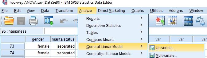
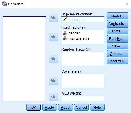
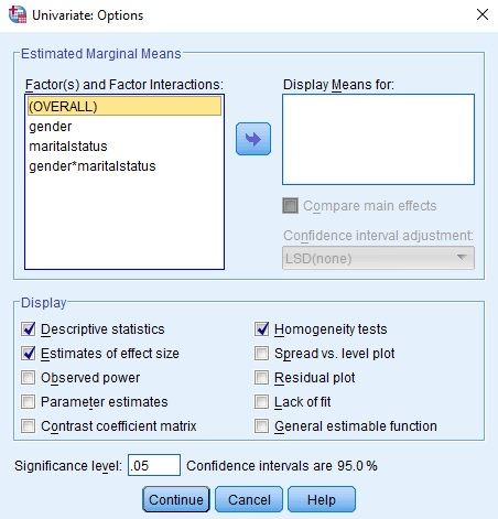
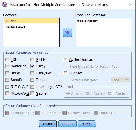
Open the Univariate Dialog
Choose Analyze, then General Linear Model, then Univariate. The dialog shows the variable list at its left and the boxes for the dependent variable and the factors at its right.
Check: Univariate takes one outcome and categorical factors. Several outcomes call for Multivariate, and the same people measured on several occasions for Repeated Measures.
Assign Happiness and Both Fixed Factors
Move happiness into Dependent Variable, and gender and maritalstatus into Fixed Factor(s). Random Factor(s), Covariate(s) and WLS Weight stay empty, and Model keeps its full factorial default, which includes the interaction.
Watch: The nominal icons beside gender and maritalstatus mark them as categories. In the output, the df of maritalstatus should be 4, one less than its five levels.
Choose Options and Tukey Post Hoc
In Options, tick Estimates of effect size, Homogeneity tests and Descriptive statistics. In Post Hoc, move maritalstatus into Post Hoc Tests for, tick Tukey under Equal Variances Assumed and select Continue.
Tip: Tukey here compares the observed marital status means, which pool both genders, on the model’s error term. It says nothing about single cells, so it answers a different question from the interaction.
Add the Interaction Profile Plot
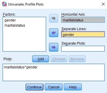
In Plots, move maritalstatus into Horizontal Axis and gender into Separate Lines, then select Add, so that maritalstatus*gender appears in the Plots box. Continue and OK run the model.
Watch: Which factor goes on the axis is only a display choice. The five-level factor on the axis gives two lines to compare, which reads more easily than five lines of two points.
Check Counts and Cell Means in the Viewer
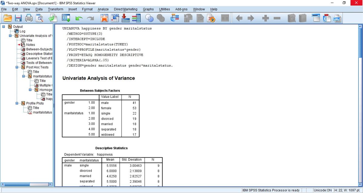
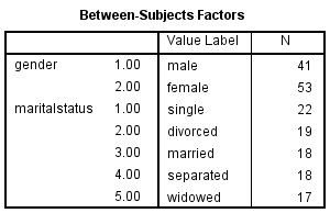
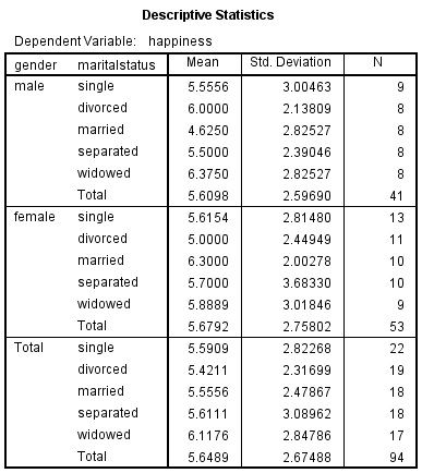
The Viewer opens with the UNIANOVA syntax log, then Between-Subjects Factors (41 male, 53 female; 22, 19, 18, 18 and 17 by status) and Descriptive Statistics, with a mean, SD and N for each of the ten cells.
Check: Cell Ns run from 8 to 13, so the design is unbalanced and the Type III sums of squares matter. The factor counts hide this, and only Descriptive Statistics shows the cells.
Read Levene's Test Before the F Rows
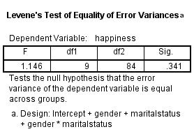
Levene’s Test of Equality of Error Variances prints F = 1.146, df1 = 9, df2 = 84 and Sig. = .341, and its footnote lists the design as Intercept + gender + maritalstatus + gender * maritalstatus.
Watch: A Sig. of .341 gives no evidence against equal error variances, and it does not show that they are equal. The largest cell SD is about 1.8 times the smallest, a ratio worth weighing beside the p.
Read the Effects Table, Tukey Rows and Plot
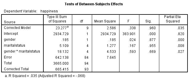
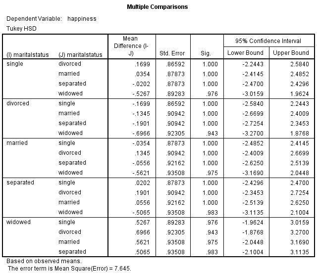
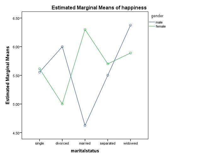
In Tests of Between-Subjects Effects, read gender * maritalstatus first (F = .593, Sig. = .669), then the two main effects. Multiple Comparisons lists the Tukey HSD pairs, and the profile plot draws the ten cell means.
Watch: With unequal cells, the three effect sums of squares (.185 + 5.109 + 18.132 = 23.426) do not add up to the Corrected Model line (23.277). That is how Type III works, not an error.
READING THE OUTPUT
Reading Cell Means, Levene and the Effects Table
For each value it lists from the SPSS output, the table gives the example figure from the video and explains how to read it in your own data.
| Output value | In the example | How to read it |
|---|---|---|
| N | Male 9, 8, 8, 8, 8; Female 13, 11, 10, 10, 9 | Cells in the order single, divorced, married, separated, widowed. They add up to 94 |
| Mean and Std. Deviation | Cell means 4.6250 to 6.3750; SDs 2.00278 to 3.68330 | Ten cell summaries on the happiness scale. Report SDs, and the means beside the interaction |
| Levene F, df1, df2, Sig. | 1.146, 9, 84 and .341 | Printed for information. With unequal cells, the F tests are most sensitive to this check |
| gender * maritalstatus | F .593, df 4, Sig. .669, partial eta squared .027 | The interaction row, read first. It tests whether the gender gap changes with marital status |
| gender | F .024, df 1, Sig. .877, partial eta squared .000 | Main effect averaged over marital status. A .000 means below .0005 |
| maritalstatus | F .167, df 4, Sig. .955, partial eta squared .008 | Main effect averaged over gender. Read only in light of the interaction row |
| Error | SS 642.138, df 84, MS 7.645 | Variation within cells, 94 cases minus 10 cells. It is the denominator of every F |
| Tukey HSD Sig. | .943 to 1.000 across the ten pairs | Observed marital status means, with the Error mean square of 7.645 named in the footnote |
COMMON MISTAKES
Slips With Post Hoc Tests, Totals and R Squared
The six slips below happen while setting up the data, working in the SPSS dialogs, reading the output or writing up, and each has a note on prevention.
Crossing Lines Read as an Interaction The male and female lines cross three times in the plot, yet the interaction F is .593. The axis spans only about 4.5 to 6.5, with no intervals, and cell means of 8 to 13 people have standard errors of roughly 0.6 to 1.2.
Gender Moved Into Post Hoc Tests For A factor with two levels has one comparison, and the F row already makes it. Only maritalstatus has three or more groups, so SPSS has nothing to add for gender and warns that no post hoc test is run.
F Tests Reported Without Cell Means A write-up that lists three F tests but not the ten cell means leaves the interaction unreadable. Give the means and SDs from Descriptive Statistics, with N per cell, next to the F rows.
Weighted Totals Taken as the Tested Means The Total rows of Descriptive Statistics weight each cell by its N, while the Type III tests compare unweighted averages of the cells. For men, 5.6098 differs slightly from the cell average of 5.6111.
Interaction Dropped After a Null Result Refitting a main-effects model after seeing p = .669 makes later tests depend on that look and changes the error term. Decide before the run whether the interaction belongs, since Model keeps it by default.
A Negative Adjusted R Squared Misread The footnote under the effects table prints R Squared = .035 and Adjusted R Squared = -.068. A negative adjusted value arises when the model F is below 1, here .338, and does not mean the run failed.
If you have already run this test, Independent Statistical Review has an OnlineSPSS statistician check the interaction, Tukey and the wording against your output.
SOURCES
Sources and Further Reading
Statements on this page draw on the literature listed below, and a line under each entry says what it is worth reading for.
Maxwell, S. E., Delaney, H. D., & Kelley, K. (2017). Designing experiments and analyzing data: A model comparison perspective (3rd ed.). Routledge.
Read this for factorial designs, interactions and simple effects.
Lakens, D. (2013). Calculating and reporting effect sizes to facilitate cumulative science: A practical primer for t-tests and ANOVAs. Frontiers in Psychology, 4, Article 863. DOI: 10.3389/fpsyg.2013.00863
Read this for how partial eta squared is defined and reported.
FREQUENTLY ASKED QUESTIONS
Menus, Simple Effects and Partial Eta Squared in the Example
Questions on this two-way ANOVA follow, from a screen that looks different in SPSS through the method and the video example to wording the result.
Why does the Univariate dialog look different in my SPSS?
The video was recorded in an older release of IBM SPSS Statistics. In release 30, IBM’s documentation still places Univariate under Analyze, General Linear Model, and lists Type III as the default sum of squares, as the video’s effects table shows. Dependent Variable, Fixed Factor(s) and the Plots and Post Hoc buttons work as shown.
What would a significant interaction change in this example?
The main effects would be averages over levels where the gender gap differs, so they could hide opposite patterns. Simple effects, gender within each marital status or the reverse, become the follow-up (Maxwell et al., 2017). In the release shown, Options has no box for them, so they need Paste and an EMMEANS line with COMPARE and an adjustment.
How large is a partial eta squared of .027 for the interaction?
It is 18.132 / (18.132 + 642.138), the interaction sum of squares over itself plus error. Gender gives .000 and marital status .008 by the same formula. Partial eta squared depends on which other factors sit in the design, so name it as partial when comparing it with other studies (Lakens, 2013).
How are F(4, 84) = 0.59 and the two main effects written up?
Interaction first. A two-way ANOVA of happiness on gender and marital status (N = 94) found no statistically significant interaction, F(4, 84) = 0.59, p = .669, partial eta squared = .027. The main effects were not significant either: gender, F(1, 84) = 0.02, p = .877; marital status, F(4, 84) = 0.17, p = .955. The ten cell means and SDs go in a table beside it.
NEXT STEP
Need a Two-Factor Design
Run or Checked?
OnlineSPSS is a statistical consultancy for researchers. Share your design and dataset, and a statistically trained Research Coordinator reviews it. The scope and one fixed project fee are confirmed before work begins.
No Commitment Required
Strictly Confidential
Fixed Project Fee
In-House PhD-Level Statisticians
Same-Day Response
Serving Researchers Since 2014