
Exploratory Factor Analysis in SPSS
Video Walkthrough of a Worked PCA Example
This exploratory factor analysis in SPSS video reduces ten mood ratings to two correlated components, using Principal components with Direct Oblimin. The page adds what that choice means, how KMO and Bartlett are read and how the pattern matrix groups items.
WATCH THE VIDEO
Exploratory Factor Analysis in SPSS, Start to Finish
Name the method as it was run. Principal components with Direct Oblimin summarizes the variance of ten ratings in two correlated components, and it is not a common-factor model (Fabrigar et al., 1999). Call the results components, or choose principal axis or maximum likelihood when latent factors are the aim.
IN SHORT
What the Video Shows in Brief
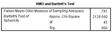
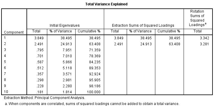
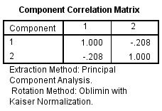
In this exploratory factor analysis in SPSS video, ten mood ratings on a 1 to 5 scale are analyzed in the Factor dialog with Principal components and Direct Oblimin rotation. The path is Analyze, Dimension Reduction, Factor. KMO is .791, two components have eigenvalues above 1 and explain 63.408% of the variance, and the two components correlate at -.208.
BEFORE YOU RUN
Checks on Ten Ratings Before Dimension Reduction
Each of the four points below is a check on the study design or the data, made before any output is produced in SPSS.
Ten Ratings on a 1 to 5 Scale Pearson correlations treat the five steps as numbers. Several items are skewed, such as scared, with 235 of 436 ratings at 1, and skew tends to shrink correlations. A polychoric matrix is the usual alternative.
Cases for Ten Items The file holds 439 cases, and 435 have all ten ratings. No fixed N is enough alone, because the size needed depends on the communalities and on how many items define each component (MacCallum et al., 1999).
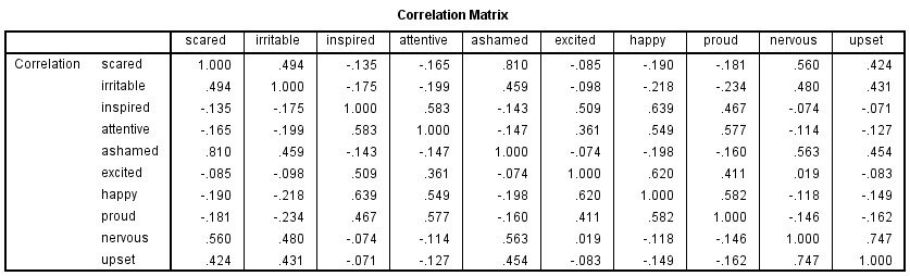
Correlations Worth Factoring Among the five negative items the correlations run from .424 to .810, and among the five positive items from .361 to .639. Across the two sets they stay between -.234 and .019, a pattern that makes two groups plausible.
Independent Respondents Each case is one respondent with ten ratings. Respondents who rated their feelings in one class or exam session can share a mood that forms a component of its own, so describe how the sample was drawn.
STEP BY STEP
Setting Up the Factor Dialog for Direct Oblimin
Screenshots of IBM SPSS show what you will see along the way. The numbered steps below give the menu path and the settings, each with a check or a tip.
Every slide pictures the SPSS screen for a single step and is numbered to match it. Labels in your version may differ a little, as the video comes from an older release.
Open the Factor Analysis Dialog
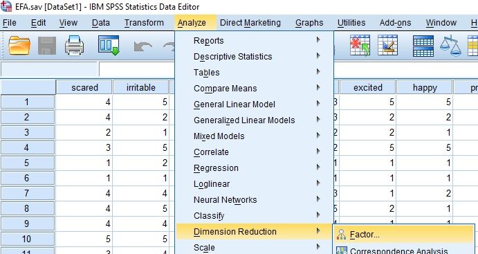
Choose Analyze, then Dimension Reduction, then Factor. A dialog named Factor Analysis opens, and its right-hand buttons are Descriptives, Extraction, Rotation, Scores and Options.
Check: Factor is the item for principal components and for common-factor models. Correspondence Analysis, listed beside it, summarizes the categories of a table and not rating items.
Move the Ten Ratings Into Variables
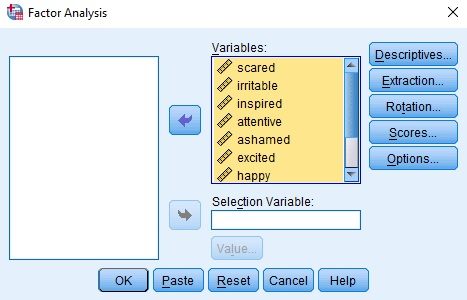
Select scared, irritable, inspired, attentive, ashamed, excited, happy, proud, nervous and upset and move them into Variables. The box scrolls, so the screenshot shows only seven of the ten.
Tip: The Selection Variable box limits the run to cases with one value of another variable, for example one random half of the sample. Here it stays empty, so every case is used.
Request KMO and Bartlett in Descriptives
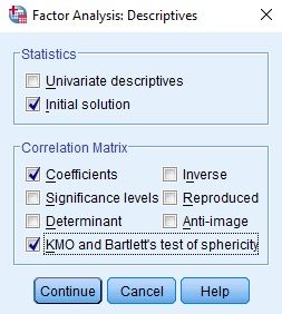
Select Descriptives. Under Statistics tick Initial solution, and under Correlation Matrix tick Coefficients and KMO and Bartlett’s test of sphericity. Then select Continue.
Tip: The Anti-image box, unticked here, adds a sampling adequacy value for each item on the diagonal. One weak item then shows up, where the overall KMO would average it away.
Choose Principal Components in Extraction
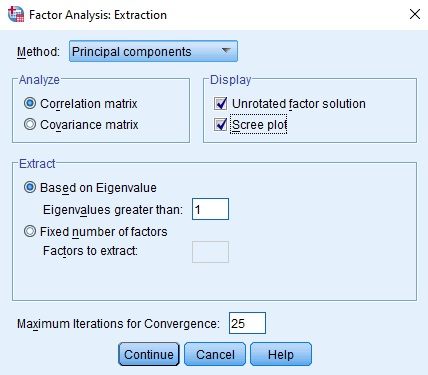
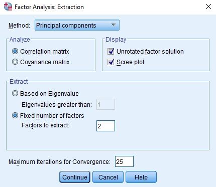
Select Extraction. Method is Principal components, Analyze is Correlation matrix, and Display has Unrotated factor solution and Scree plot ticked. Extract reads Based on Eigenvalue, with Eigenvalues greater than 1.
Watch: Covariance matrix in the Analyze box would let items with larger variances weigh more. Correlation matrix puts every rating on the same footing, which suits items from one scale.
Set Oblimin, Pairwise Exclusion and Sorting
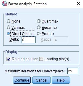
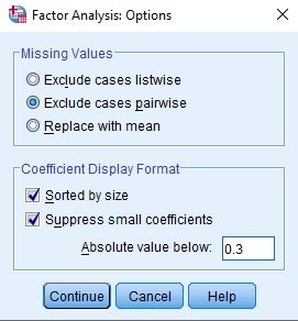
In Rotation select Direct Oblimin with Delta 0 and tick Rotated solution. In Options choose Exclude cases pairwise, tick Sorted by size and Suppress small coefficients below .3, then select OK.
Tip: Delta 0 is the default, which IBM Support calls the most oblique setting, and more negative values make the components less oblique. Oblimin lets the components correlate, where Varimax would not.
Read KMO, Variance Explained and Scree
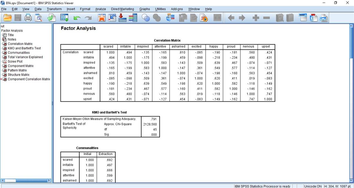
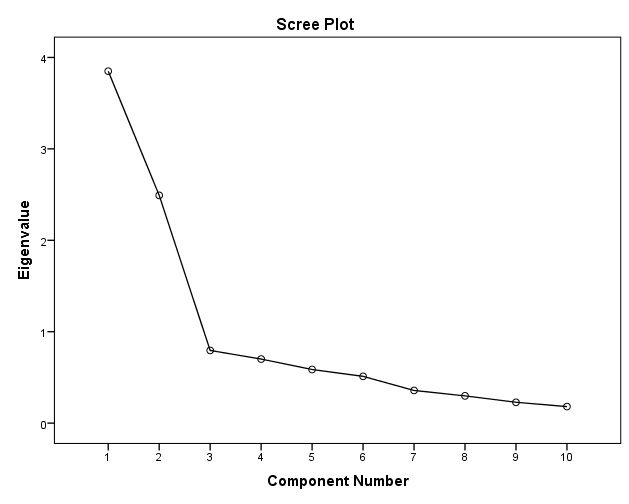
The Viewer lists Correlation Matrix, KMO and Bartlett’s Test, Communalities, Total Variance Explained and Scree Plot, then the matrices. KMO reads .791, and the first eigenvalues are 3.849, 2.491 and .795.
Check: The Initial Eigenvalues column adds up to 10, one unit for each standardized item. That is why Cumulative % ends at 100.000 on the tenth component.
Fix Two Components and Read the Matrices
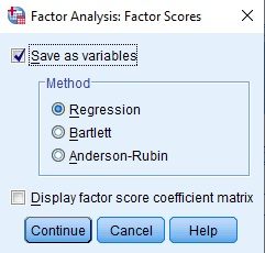
Reopen Extraction, choose Fixed number of factors with 2, and in Scores tick Save as variables with the Regression method. Pattern Matrix, Structure Matrix and Component Correlation Matrix follow in the output.
Watch: Based on Eigenvalue already kept two components, so this run reproduces the first solution. A fixed number matters when your judgment about the count differs from the eigenvalue rule.
READING THE OUTPUT
Reading KMO, Eigenvalues and the Pattern Matrix
For each value it lists from the SPSS output, the table gives the example figure from the video and explains how to read it in your own data.
| Output value | In the example | How to read it |
|---|---|---|
| KMO Measure of Sampling Adequacy | .791 | Compares the correlations with the partial correlations across all ten items. It describes the matrix, not the number of cases |
| Bartlett’s Test of Sphericity | 2128.560, df 45, Sig. .000 | Tests whether the correlation matrix is an identity matrix |
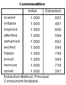
| Communalities, Extraction | .497 (irritable) to .749 (happy) | The share of each item’s variance held by the two components. The initial 1.000 is how components start |
| Initial Eigenvalues | 3.849 and 2.491, then .795 | The variance of each component in item units. Cumulative % reaches 63.408 at component 2 |
| Rotation Sums of Squared Loadings | 3.342 and 3.281 | Sums after rotation, printed without a cumulative percentage because correlated components overlap |
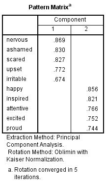
| Pattern Matrix | Component 1 from nervous .869 to irritable .674; Component 2 from happy .856 to proud .744 | Loadings after Oblimin. Cells below .3 are blank, and no item has a second loading above it |
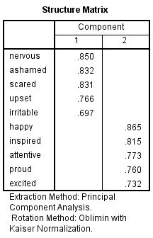
| Structure Matrix | nervous .850, happy .865 | The correlation of each item with each component. It differs from the pattern values because the components correlate |
| Component Correlation Matrix | -.208 | The correlation between the two components, weak and negative |
COMMON MISTAKES
Slips With Bartlett, Blank Loadings and Rotated Variance
Six mistakes follow, each tied to a stage (data setup, SPSS dialogs, output or write-up) and each paired with a brief note on how to avoid it.
Bartlett's p Read as a Green Light A Sig. of .000 is p < .001, and with 435 cases a modest correlation matrix would also reach it. It says little about whether components exist, so judge the matrix from the correlations and KMO.
Blank Cells Read as Zero Loadings Suppress small coefficients at .3 blanks every value below .30. A blank is a small loading and not a zero, and a cross-loading of .29 stays invisible, so rerun without suppression before calling the structure clean.
Component Names Treated as Findings Negative feelings and positive feelings are labels the researcher adds after reading the pattern matrix. SPSS prints Component 1 and Component 2 only, so name them as an interpretation and not as a result.
Rotation Picked After the Loadings Direct Oblimin was set before the run, because correlated components are plausible for mood items. Switching to Varimax afterwards because the loadings look tidier lets the result choose the method.
Saved Scores Treated as Measured Values Save as variables adds one regression score per component to the data file. They are estimates that depend on the extraction and rotation settings, so name those settings wherever the scores are used.
Variance Added Across Rotated Components The rotation sums of 3.342 and 3.281 add to 6.623, more than the 6.340 held by two components, so they are never summed. Quote the 63.408% from Total Variance Explained.
If you have already run this test, Independent Statistical Review has an OnlineSPSS statistician check the extraction, the rotation and the wording against your output.
SOURCES
Sources and Further Reading
Statements on this page draw on the literature listed below, and a line under each entry says what it is worth reading for.
Fabrigar, L. R., Wegener, D. T., MacCallum, R. C., & Strahan, E. J. (1999). Evaluating the use of exploratory factor analysis in psychological research. Psychological Methods, 4(3), 272-299. DOI: 10.1037/1082-989X.4.3.272
Read this for the decisions that shape an exploratory analysis.
MacCallum, R. C., Widaman, K. F., Zhang, S., & Hong, S. (1999). Sample size in factor analysis. Psychological Methods, 4(1), 84-99. DOI: 10.1037/1082-989X.4.1.84
Read this for the factors that set the sample size a factor analysis needs.
Hayton, J. C., Allen, D. G., & Scarpello, V. (2004). Factor retention decisions in exploratory factor analysis: A tutorial on parallel analysis. Organizational Research Methods, 7(2), 191-205. DOI: 10.1177/1094428104263675
Read this for how parallel analysis guides the number of factors.
FREQUENTLY ASKED QUESTIONS
Menus, Retention and Matrices in the Example
Four questions are answered here. They deal with the SPSS screens, the method behind this analysis, the example in the video and how to report what it shows.
Why does the Factor Analysis dialog look different in my SPSS?
The video was recorded in an older release of IBM SPSS Statistics. IBM’s documentation for the FACTOR command lists principal components as the default extraction, with principal axis factoring and maximum likelihood among the others, and varimax as the command’s default rotation. The video’s Direct Oblimin was therefore a deliberate choice.
Does the eigenvalue rule settle the number of components?
No, it is one input to a judgment. Here the third eigenvalue is .795 and the scree plot bends after the second point. Computed outside SPSS, parallel analysis on 1,000 random normal datasets of 435 cases and ten items gives 95th percentile eigenvalues near 1.31, 1.22 and 1.15, so only two observed eigenvalues exceed them (Hayton et al., 2004).
Which matrix is quoted when the components correlate?
Both are printed. Pattern coefficients show what a component adds to an item with the other held constant, and structure coefficients are the plain item-component correlations. With r = -.208 they differ little: nervous reads .869 and .850, happy .856 and .865. Say which matrix a loadings table quotes.
How are KMO .791 and two components written up?
State the method exactly and the retention basis. A principal components analysis with Direct Oblimin rotation was run on ten items (KMO = .79, Bartlett’s chi-square(45) = 2128.56, p < .001). Two components, kept on the eigenvalues, the scree plot and parallel analysis, accounted for 63.41% of the variance and correlated at -.21.
NEXT STEP
Need an Item Structure Explored,
Run or Checked?
OnlineSPSS is a statistical consultancy for researchers. Share your design and dataset, and a statistically trained Research Coordinator reviews it. The scope and one fixed project fee are confirmed before work begins.
No Commitment Required
Strictly Confidential
Fixed Project Fee
In-House PhD-Level Statisticians
Same-Day Response
Serving Researchers Since 2014