
Binary Logistic Regression in SPSS
Video Walkthrough of a Worked Odds Example
This binary logistic regression in SPSS video predicts whether people like going to work from their hours of sleep, in one dialog. The page adds how the event is coded, what Block 0 holds and why Exp(B) is an odds ratio and not a change in probability.
WATCH THE VIDEO
Binary Logistic Regression in SPSS, Start to Finish
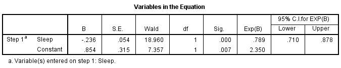
Quote the odds ratio with its interval and set the classification table beside it, not a pseudo R squared alone. Here Exp(B) is .789 with 95% CI [.710, .878], so in the fitted model each extra hour of sleep multiplies the odds of liking work by about .79. Yet 62.0% of cases are classified correctly against 60.5% for the constant alone, so a small p-value is not the same as good prediction.
IN SHORT
What the Video Shows in Brief
In this binary logistic regression in SPSS video, the answer to “Do you like going to work” (no or yes) is modeled from hours of sleep for 266 of 271 cases. The path is Analyze, Regression, Binary Logistic. Sleep has B = -.236 and Exp(B) = .789, 95% CI [.710, .878], p < .001: statistically significant, and the interval excludes 1.
BEFORE YOU RUN
Checks on a Yes-No Outcome Before Logistic Regression
The four points below concern your study design and your data. Settle each one first, then run this logistic regression in SPSS.
Two Outcome Categories The outcome is no or yes to liking work, and the model describes the log odds of the category coded 1. Cutting a rating scale into two groups to fit this model discards information and makes the result depend on the cut.
Cases in the Rarer Category The information sits in the 105 yes cases among 266, not in the total N. The rule of thumb of 10 events per predictor was examined in a simulation study (Peduzzi et al., 1996), and one predictor is far inside it.
A Straight Line on the Logit Scale The model assumes the log odds shift in a straight line with hours. Counted in the data file, the share of yes stays near 43% to 50% from 2 to 7 hours, then falls to 2 of 32 at 9 hours, a bend that one Exp(B) averages over.
Independent Cases Each person is one row, and the rows are unrelated. Several rows per person, or pupils nested in classes, break this, and the p-values then claim more precision than the data hold.
STEP BY STEP
Entering Work and Sleep in the Logistic Regression Dialog
Follow the numbered steps below through IBM SPSS, with screenshots as you go: each step gives the menu path, the settings to pick and a check or tip.
Each slide shows the SPSS screen for one step and carries its step number. The video was recorded in an older release, so labels on your screen may differ slightly.
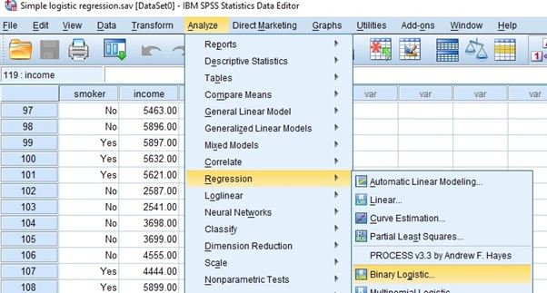
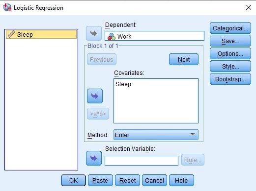
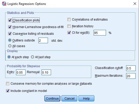
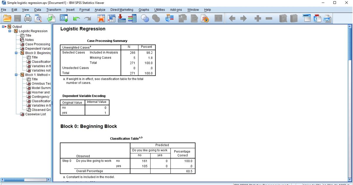
Open the Logistic Regression Dialog
Choose Analyze, then Regression, then Binary Logistic. The window that opens is titled Logistic Regression and takes one two-category outcome.
Check: An outcome with three or more unordered categories belongs in Multinomial Logistic, listed in the same Regression submenu. Binary Logistic needs exactly two outcome categories.
Place Work and Sleep in the Boxes
Move Work into Dependent and Sleep into Covariates. The dialog reads Block 1 of 1 and keeps Method on Enter, so Sleep goes into the model in one step.
Watch: The other Method choices add or drop predictors step by step on a statistical criterion. They suit exploratory prediction and not a model with one predictor named in advance.
Tick Hosmer-Lemeshow and CI for exp(B)
Select Options and tick Classification plots, Hosmer-Lemeshow goodness-of-fit, Casewise listing of residuals and CI for exp(B) at 95%. The cutoff stays at .5 and Display stays on At each step. Then Continue and OK.
Tip: Without CI for exp(B), the coefficients table prints Exp(B) as a point estimate only. The interval is the uncertainty of the odds ratio, so tick it before the run.
Find Block 0 in the Viewer
The outline lists Case Processing Summary, Dependent Variable Encoding, Block 0 with its Classification Table and Variables in the Equation, then Block 1 with Omnibus Tests, Model Summary and the later tables.
Watch: Block 0 is the model with the constant alone, so its tables describe a baseline with no predictor. The Sleep results begin at Block 1.
Check the Cases and the Coding
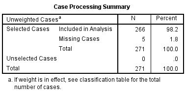
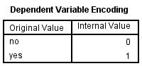
Case Processing Summary counts 266 cases in the analysis, 5 missing and 271 in total. Dependent Variable Encoding maps the original value no to 0 and yes to 1, which is the order the model uses.
Check: A missing Work or Sleep value drops the case without a message. In the data file, two cases have no Work value and three have no Sleep value, which accounts for the 5 missing.
Compare Block 0 With the Fitted Model
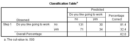
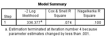
Classification Table, Step 1, reads 131 and 30 for no, 71 and 34 for yes, 62.0% correct. Model Summary gives -2 Log likelihood 336.377, Cox and Snell .074 and Nagelkerke .100.
Tip: Hold the Step 1 table against the Block 0 table, where all 266 cases are predicted no and 60.5% are correct. The gain from Sleep is the difference between those two figures.
Read Variables in the Equation
The Sleep row gives B = -.236, S.E. .054, Wald 18.960 on 1 df, Sig. .000, Exp(B) .789 and its 95% interval .710 to .878. The Constant row reads B = .854 and Exp(B) 2.350.
Watch: Exp(B) belongs to one extra hour. Two extra hours multiply the odds by .789 squared, about .62, so state the unit before quoting the odds ratio.
READING THE OUTPUT
Reading Block 0, Model Summary and the Coefficients
Each value below comes from the SPSS output. Its row shows the figure in the video example, then how to interpret it when the data are your own.
| Output value | In the example | How to read it |
|---|---|---|
| Block 0 Classification Table | 161 no, 105 yes, 60.5% correct | The baseline: the constant alone predicts no for everyone, so a model must beat 60.5% to add anything here |
| Classification Table, Step 1 | 131, 30, 71, 34; 81.4%, 32.4%, 62.0% | Cutoff .500. Only 64 cases are predicted yes, and 34 of the 105 true yes cases are found |
| Cox & Snell and Nagelkerke | .074 and .100 | Pseudo R squared values from the likelihood. Nagelkerke rescales Cox and Snell to reach 1 (Nagelkerke, 1991) and is not variance explained |
| B and S.E. | Sleep -.236 (.054), Constant .854 (.315) | Log odds scale. The negative sign means more sleep goes with lower odds of yes |
| Wald and Sig. | 18.960, 1 df, .000 | Wald test for Sleep on 1 df |
| Exp(B) and its 95% CI | .789, .710 to .878 | The odds ratio per extra hour, about 21% lower odds. The interval excludes 1 |
| Omnibus Tests of Model Coefficients | Not among the screenshots | The test of the whole model. Look for its chi-square in your own output |
| Hosmer and Lemeshow Test | Printed after Model Summary | Observed against expected counts in groups of predicted risk, printed as a chi-square, df and Sig. for Step 1 |
COMMON MISTAKES
Slips With Categorical Predictors, Block 0 and Exp(B)
These six mistakes arise in the data setup, the SPSS dialogs, the output or the write-up, and each comes with a short note on how to avoid it.
Categorical Predictors Left as Numbers A predictor with three coded groups belongs under the Categorical button. Left in Covariates, it is read as one numeric slope, and its single Exp(B) hides the contrasts between the groups.
Block 0 Quoted as the Result Block 0 prints a Classification Table of 60.5% and a coefficients table with only the constant. They describe the baseline, so quote the Block 1 tables for the model.
The Cutoff Treated as Part of the Model The classification cutoff of .5 only turns predicted probabilities into no or yes. Changing it moves cases between cells of the Classification Table and leaves B, Exp(B) and the p-values unchanged.
The Wald Test Trusted at Its Limits Sig. in Variables in the Equation comes from a Wald test. With very large coefficients or near-separation the Wald value shrinks, so check a large p against the likelihood-ratio test, here the Omnibus Tests chi-square.
A Large Hosmer-Lemeshow p as Proof of Fit A Sig. above .05 gives no evidence of poor fit in the groups used. It does not show that the model fits, and it depends on the grouping and the N, so read it with the observed and expected counts.
The Wrong Category Taken as the Event The higher code is the event, here 1 for yes. Coded the other way, B would be +.236 and Exp(B) 1.267, the same finding told as the odds of no. Read Dependent Variable Encoding before the signs.
If you have already run this test, Independent Statistical Review has an OnlineSPSS statistician check the event coding, Exp(B) and the wording against your output.
SOURCES
Sources and Further Reading
A note under each reference says what to read it for, and every reference listed supports a statement on this page.
Peduzzi, P., Concato, J., Kemper, E., Holford, T. R., & Feinstein, A. R. (1996). A simulation study of the number of events per variable in logistic regression analysis. Journal of Clinical Epidemiology, 49(12), 1373-1379. DOI: 10.1016/S0895-4356(96)00236-3
Read this for what a simulation found about events per variable.
Nagelkerke, N. J. D. (1991). A note on a general definition of the coefficient of determination. Biometrika, 78(3), 691-692. DOI: 10.1093/biomet/78.3.691
Read this for how Cox and Snell's R squared is rescaled to reach 1.
FREQUENTLY ASKED QUESTIONS
Menus, Whole-Model Tests and Odds in the Example
These answers explain why the SPSS screens may look different from the video, then take up the method, the example figures and how to write the result up.
Why does the Logistic Regression dialog look different in my SPSS?
The video was recorded in an older release of IBM SPSS Statistics. Its dialog has Categorical, Save, Options, Style and Bootstrap buttons. IBM’s release 23 page for Options lists the same Statistics and Plots items, a classification cutoff from .01 to .99 and a Display choice of At each step or At last step.
Where is the test of the whole model in the video?
The Viewer outline lists Omnibus Tests of Model Coefficients, but no screenshot of it is used, so no value is quoted from it. Computed outside SPSS from the data, the likelihood-ratio chi-square is about 20.50 on 1 df, the baseline -2 log likelihood of 356.88 minus 336.38, with p below .001.
How does Exp(B) of .789 relate to the probability of yes?
Exp(B) multiplies the odds by the same factor for every extra hour, so the probability falls by different amounts. Computed outside SPSS from B = -.236 and the constant .854, the predicted probability of yes is about .54 at 3 hours, .36 at 6 hours and .22 at 9 hours. Give probabilities only for hours that you name.
How are Exp(B) = .789 and 62.0% correct written up?
Name the outcome, the odds ratio with its interval and the baseline. More hours of sleep went with lower odds of liking work, B = -.236, Wald chi-square(1) = 18.96, p < .001, Exp(B) = .789, 95% CI [.710, .878], Nagelkerke R2 = .100. The model classified 62.0% of 266 cases correctly, against 60.5% for the constant alone.
NEXT STEP
Need a Two-Category Outcome Modeled,
Run or Checked?
OnlineSPSS is a statistical consultancy for researchers. Share your design and dataset, and a statistically trained Research Coordinator reviews it. The scope and one fixed project fee are confirmed before work begins.
No Commitment Required
Strictly Confidential
Fixed Project Fee
In-House PhD-Level Statisticians
Same-Day Response
Serving Researchers Since 2014