
Repeated Measures ANOVA in SPSS
Video Walkthrough of a Worked Time Example
This repeated measures ANOVA in SPSS video follows the math scores of 51 people across three occasions in the GLM dialogs. The page adds how the Time factor is defined, which sphericity row to quote and what a partial eta squared of .897 says.
WATCH THE VIDEO
Repeated Measures ANOVA in SPSS, Start to Finish
Settle the sphericity route before the output is opened, and name it in the report: the sphericity-assumed row, a corrected row and the multivariate tests answer the Time question under different conditions (Keselman et al., 2001). A corrected row, which multiplies both df by epsilon (Greenhouse & Geisser, 1959), is a sound planned default. Here epsilon is .983, so the corrected df of 1.97 and 98.26 barely differ from 2 and 100, and both rows give p < .001.
IN SHORT
What the Video Shows in Brief
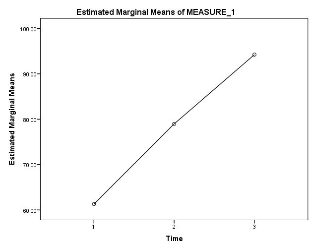
In this repeated measures ANOVA in SPSS video, 51 people’s math scores are compared before training, after one month and after two months, with Time as a within-subjects factor of three levels. The path is Analyze, General Linear Model, Repeated Measures, then Define Factor(s). The Greenhouse-Geisser row gives F(1.97, 98.26) = 437.14, p < .001, with partial eta squared .897, and the means rise from 61.27 to 78.96 to 94.24.
BEFORE YOU RUN
Checks on Within-Subjects Data Before Define Factor(s)
Four points about your design and your data come first. Each of them is decided before this repeated measures ANOVA is run in SPSS.
One Row per Person Each person fills one row with three scores, so the scores within a row are related and different people are independent. Anyone missing a score on one occasion leaves the analysis, and classes or clinics call for a multilevel model.
Continuous Scores on One Scale The score must mean the same thing at each occasion, in the same units on an interval scale. Ordinal scores point to the Friedman test, and two occasions only to the paired samples t-test.
Shape of the Change Scores The F tests concern differences between occasions, so look at the three difference scores or the residuals for outliers and strong skew, not only at the raw columns. A histogram of each shows whether a few people drive the result.
A Design Behind the Time Effect The occasions follow one another in a fixed order and no group goes untrained, so a rise over time mixes training with practice and other events. The design cannot attribute the change to the training alone.
STEP BY STEP
Defining Time in the Repeated Measures Dialogs
Menu path, settings and a check or tip: the numbered steps below give all three for every step of this repeated measures ANOVA, with screenshots from IBM SPSS.
The slides follow the step numbers, each one showing the SPSS screen for that step. The video was made in an older release, so some labels on your screen may differ.
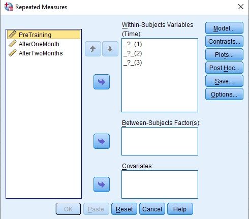
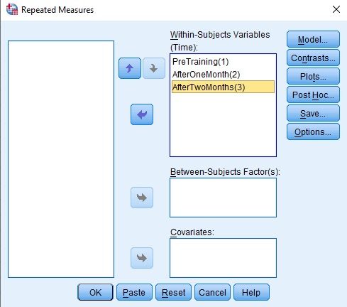
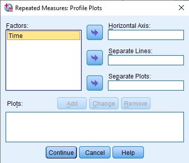
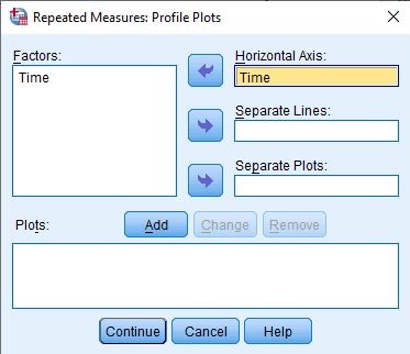
Open the Repeated Measures Dialog
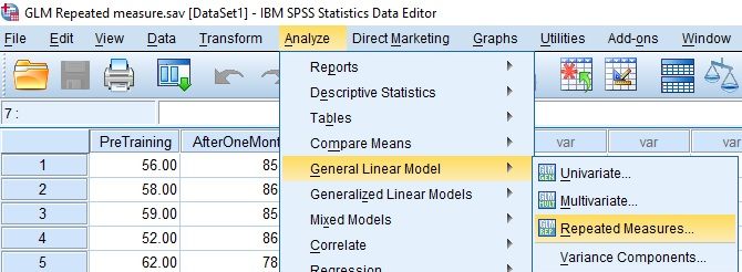
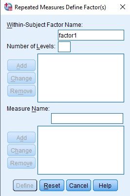
Choose Analyze, then General Linear Model, then Repeated Measures. The first window to open is Repeated Measures Define Factor(s), with factor1 filled in as the name and no levels yet.
Check: Univariate takes one outcome column and categorical factors only. Three scores of the same people sit in three columns, so they belong in Repeated Measures.
Define the Time Factor With Three Levels
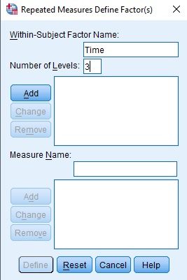
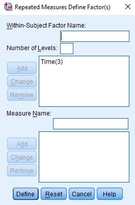
Replace factor1 with Time, type 3 in Number of Levels and select Add, so that Time(3) appears in the list. Then select Define to open the main dialog.
Watch: The number of levels must equal the number of score columns, here three. A wrong count leaves an empty slot, or a score with no slot, in the next window, and OK stays grayed out until every slot is filled.
Fill the Within-Subjects Variables Slots
Move PreTraining, AfterOneMonth and AfterTwoMonths into the slots marked _?_(1), _?_(2) and _?_(3). The Between-Subjects Factor(s) and Covariates boxes stay empty in this one-factor design.
Check: The number in brackets is the level. Level 1 must be the earliest occasion, because the output labels and the sign of every pairwise difference follow that order.
Set the Profile Plot and the Options
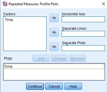
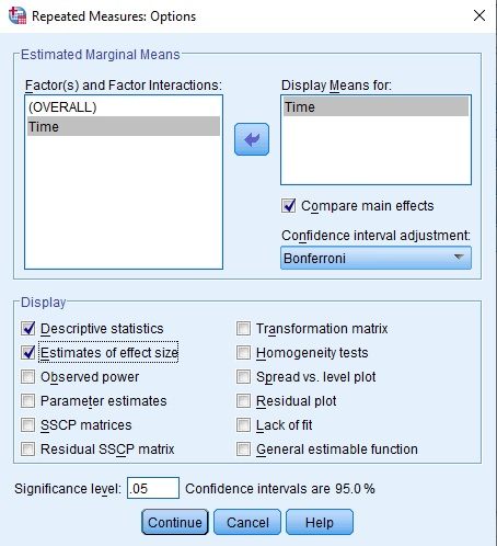
In Plots, move Time to Horizontal Axis and select Add. In Options, move Time to Display Means for, tick Compare main effects with Bonferroni, and tick Descriptive statistics and Estimates of effect size.
Tip: The default adjustment, LSD(none), would leave the three pairs unadjusted. Choose Bonferroni or Sidak before the run, so the adjustment is a planned choice and not one made after the means are seen.
Check the Factor Levels and Descriptives
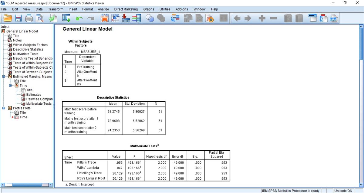
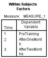
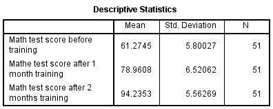
The Viewer opens with General Linear Model, then Within-Subjects Factors, which maps levels 1, 2 and 3 to PreTraining, AfterOneMonth and AfterTwoMonths. Descriptive Statistics shows N = 51 in every row.
Check: One row label reads Mathe test score after 1 month training, a typo carried over from the variable label. Correct labels in Variable View before tables are copied into a report.
Read Mauchly's Test of Sphericity
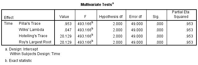
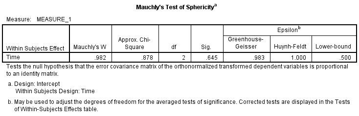
Multivariate Tests gives Wilks’ Lambda .047 and F = 493.166 on 2 and 49 df, without assuming sphericity. Mauchly’s table gives W = .982, Sig. = .645 and epsilon estimates of .983, 1.000 and .500.
Watch: A Sig. of .645 gives no evidence against sphericity, which is a weaker statement than showing that it holds. The SDs of the three change scores, 8.28, 7.42 and 8.18, show whether they are similar.
Read the Corrected Row, Pairs and Plot
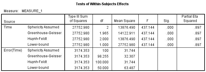
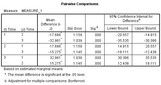
In Tests of Within-Subjects Effects, the Time rows share F = 437.144 and Sig. .000, with df 2 and 100 assumed or 1.965 and 98.255 under Greenhouse-Geisser. Pairwise Comparisons lists the pairs, and the plot draws the three means.
Tip: Report the df of the row you chose, 1.965 and 98.255 for Greenhouse-Geisser or 2 and 100 for sphericity assumed. The F is the same in every row because a correction changes only the df and so the p-value.
READING THE OUTPUT
Reading Mauchly, the Effects Table and Pairwise Rows
Row by row, the table names a value in the SPSS output for this repeated measures ANOVA, its figure in the video example and how to read it in your data.
| Output value | In the example | How to read it |
|---|---|---|
| Mean and Std. Deviation | 61.2745 (5.80027), 78.9608 (6.52062), 94.2353 (5.56269), N = 51 | PreTraining, AfterOneMonth and AfterTwoMonths in score points. Report the SD, not a standard error |
| Multivariate Tests, Wilks’ Lambda | .047, F 493.166, df 2 and 49, Sig. .000, partial eta squared .953 | Needs no sphericity. All four rows give the same F here, and its partial eta squared differs from the univariate table |
| Mauchly’s W and Sig. | .982, chi-square .878, df 2 and .645 | A check on sphericity, printed for information. Its power depends on N, so read epsilon for the size of any departure |
| Epsilon | Greenhouse-Geisser .983, Huynh-Feldt 1.000, Lower-bound .500 | The factor that shrinks both df. 1 means no departure, and .500 is the lowest possible with three levels |
| Time, Sphericity Assumed | SS 27752.980, df 2, MS 13876.490, F 437.144, Sig. .000 | The uncorrected row. Partial eta squared .897 is this SS over itself plus the Error SS |
| Time, Greenhouse-Geisser | df 1.965, MS 14122.911, F 437.144, Sig. .000 | Same F with df multiplied by .983. Error(Time) has df 98.255 and MS 32.307 |
| Pairwise Comparisons, 1 vs 2 and 1 vs 3 | -17.686 [-20.557, -14.815] and -32.961 [-35.535, -30.386] | Mean Difference (I-J) with its Bonferroni 95% CI. Sig. .000 is p < .001 |
| Pairwise Comparisons, 2 vs 3 | -15.275 [-18.111, -12.438] | Each pair appears in both directions, so the signs flip, and the adjustment covers three comparisons |
COMMON MISTAKES
Slips With Wide Data, Pairs and Partial Eta Squared
Some mistakes start in the data setup, others in the SPSS dialogs, the output or the write-up. Six of them follow, each with a short note on avoiding it.
Long-Format Data in a Wide Dialog Within-Subjects Variables wants three separate columns. Stacked data, with one score column and a code for the occasion, must be restructured so that each person has one row before the slots can be filled.
Partial Eta Squared From the Wrong Table Multivariate Tests prints .953 and Tests of Within-Subjects Effects prints .897 for the same Time effect. Quote the value from the table that holds the F you report, and say which one it is.
A Ceiling Left Unplotted Nine of the 51 scores after two months equal 100, the highest value in the file, while no earlier score exceeds 88. If 100 is the test maximum, plot the scores, since a ceiling compresses the spread.
Six Pairwise Rows Read as Six Tests Pairwise Comparisons lists each pair in both directions, but Bonferroni adjusts for three comparisons. Report the three pairs once each, giving every mean difference with its interval instead of all six rows.
A Zero p Value Quoted Sig. .000 is a rounded p, not zero. Write p < .001 for the F test and for each of the three pairs; a p printed as .000 only says it is below .0005 in either table.
A Plot Axis Read Without Its Scale The profile plot's vertical axis runs from about 60 to 100, not from zero, and it shows no interval around the three points. Read the means and the pairwise intervals from the tables, not from the slope.
If you have already run this test, Independent Statistical Review has an OnlineSPSS statistician check sphericity, the pairs and the effect size against your output.
SOURCES
Sources and Further Reading
The reading below supports what this page says about this repeated measures ANOVA, and a line under each entry notes what to read it for.
Greenhouse, S. W., & Geisser, S. (1959). On methods in the analysis of profile data. Psychometrika, 24(2), 95-112. DOI: 10.1007/BF02289823
Read this for the degrees-of-freedom adjustment behind epsilon.
Keselman, H. J., Algina, J., & Kowalchuk, R. K. (2001). The analysis of repeated measures designs: A review. British Journal of Mathematical and Statistical Psychology, 54(1), 1-20. DOI: 10.1348/000711001159357
Read this for why a report should name its repeated measures approach.
Lakens, D. (2013). Calculating and reporting effect sizes to facilitate cumulative science: A practical primer for t-tests and ANOVAs. Frontiers in Psychology, 4, Article 863. DOI: 10.3389/fpsyg.2013.00863
Read this for how partial and generalized eta squared are defined.
FREQUENTLY ASKED QUESTIONS
Menus, Multivariate Rows and Effect Size in the Example
From the SPSS menus on your screen to the final write-up, the questions here follow this analysis, taking in the method and the video example.
Why does the Repeated Measures dialog look different in my SPSS?
The video was recorded in an older release of IBM SPSS Statistics. IBM’s release 30 page keeps Repeated Measures under Analyze and General Linear Model, with the Define Factor(s) step. In current releases, Display Means for and Compare main effects sit under a separate EM Means button, not in Options. Mauchly’s test still prints automatically.
Why do Multivariate Tests and the within-subjects table both test Time?
They are two approaches to one question. Multivariate Tests does not assume sphericity but needs enough people for the number of occasions, while the within-subjects table assumes it unless a corrected row is read. Here both give p < .001 and the same decision, so name the approach reported rather than the p-value alone (Keselman et al., 2001).
What does a partial eta squared of .897 say about Time?
It is the Time sum of squares over Time plus Error, 27752.98 / (27752.98 + 3174.35), so it leaves out the variation between people. Adding the between-person sum of squares, the Error row of Tests of Between-Subjects Effects (about 2180.90), to the denominator gives a generalized eta squared near .84 (Lakens, 2013). Say which one you quote.
How is F(1.97, 98.26) = 437.14 reported with the three pairs?
Name the correction, the means and the pairs. With Greenhouse-Geisser, Time was statistically significant, F(1.97, 98.26) = 437.14, p < .001, partial eta squared = .897 (n = 51). Bonferroni-adjusted differences, 1 vs 2: -17.69, 95% CI [-20.56, -14.82]; 1 vs 3: -32.96 [-35.54, -30.39]; 2 vs 3: -15.27 [-18.11, -12.44].
NEXT STEP
Need a Repeated Measures Model
Run or Checked?
OnlineSPSS is a statistical consultancy for researchers. Share your design and dataset, and a statistically trained Research Coordinator reviews it. The scope and one fixed project fee are confirmed before work begins.
No Commitment Required
Strictly Confidential
Fixed Project Fee
In-House PhD-Level Statisticians
Same-Day Response
Serving Researchers Since 2014