
Two-Way MANOVA in SPSS
Video Walkthrough of a Worked Training Example
This two-way MANOVA in SPSS video tests whether Gender, Training and their interaction relate to the English, Math and History scores as a set. The page adds the order of reading, what the Options choice leaves out of the output, and the follow-up rows.
WATCH THE VIDEO
Two-Way MANOVA in SPSS, Start to Finish
Read the Gender * Training row before either main effect, and name the multivariate statistic before the output is opened. Here the interaction is not statistically significant under any of the four statistics, so Training is read across both genders. For Training the four statistics now differ, and Pillai’s trace is the most robust of them when assumptions are doubtful (Olson, 1974).
IN SHORT
What the Video Shows in Brief
In this two-way MANOVA in SPSS video, English, Math and History results of 109 participants are compared across Gender (male 56, female 53) and Training (1, 2 and 3 months). The path is Analyze, General Linear Model, Multivariate, with Gender and Training as Fixed Factors. The interaction is not statistically significant (Wilks’ lambda = .950, F(6, 202) = 0.88, p = .512), while Training is (Wilks’ lambda = .848, F(6, 202) = 2.89, p = .010).
BEFORE YOU RUN
Cells, Interaction and Covariances Before Multivariate
Each of the four points below is a check on the study design or the data, made before any output is produced in SPSS.
Independent Cases in Each Cell Each participant falls in one Gender and Training cell and appears once. The same people tested after 1, 2 and 3 months would make Training a within-subjects factor, which needs Repeated Measures instead.
Cell Sizes and Balance Six cells of 14 to 22 cases leave the design unbalanced, though every cell exceeds the three outcomes. Very small or empty cells weaken the multivariate tests and make the interaction hard to estimate.
Outcomes as One Set The three scores enter together because the question concerns all of them. Where each score has its own research question, a separate two-way ANOVA per score answers it more directly.
Covariance Matrices Across Six Cells Equal covariance matrices matter more when cells are unequal, and the History SDs run from 11.01 to 19.70 across the cells. That spread is worth a look before the joint tests are trusted.
STEP BY STEP
Entering Two Fixed Factors in the Multivariate Dialog
Screenshots of IBM SPSS show what you will see along the way. The numbered steps below give the menu path and the settings, each with a check or a tip.
Each slide shows the SPSS screen for one step and carries its step number. The video was recorded in an older release, so labels on your screen may differ slightly.
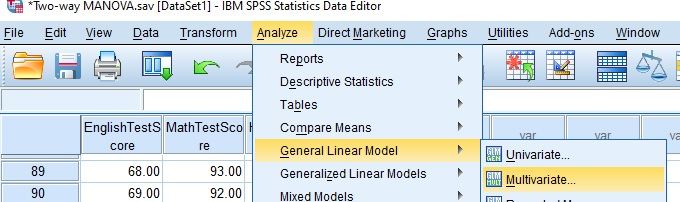
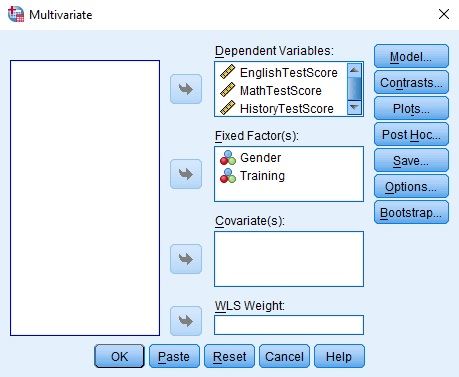
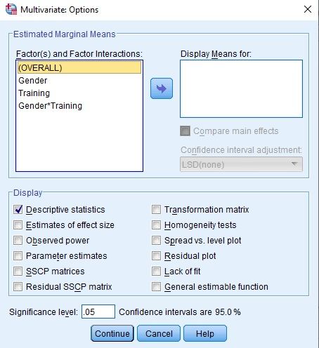
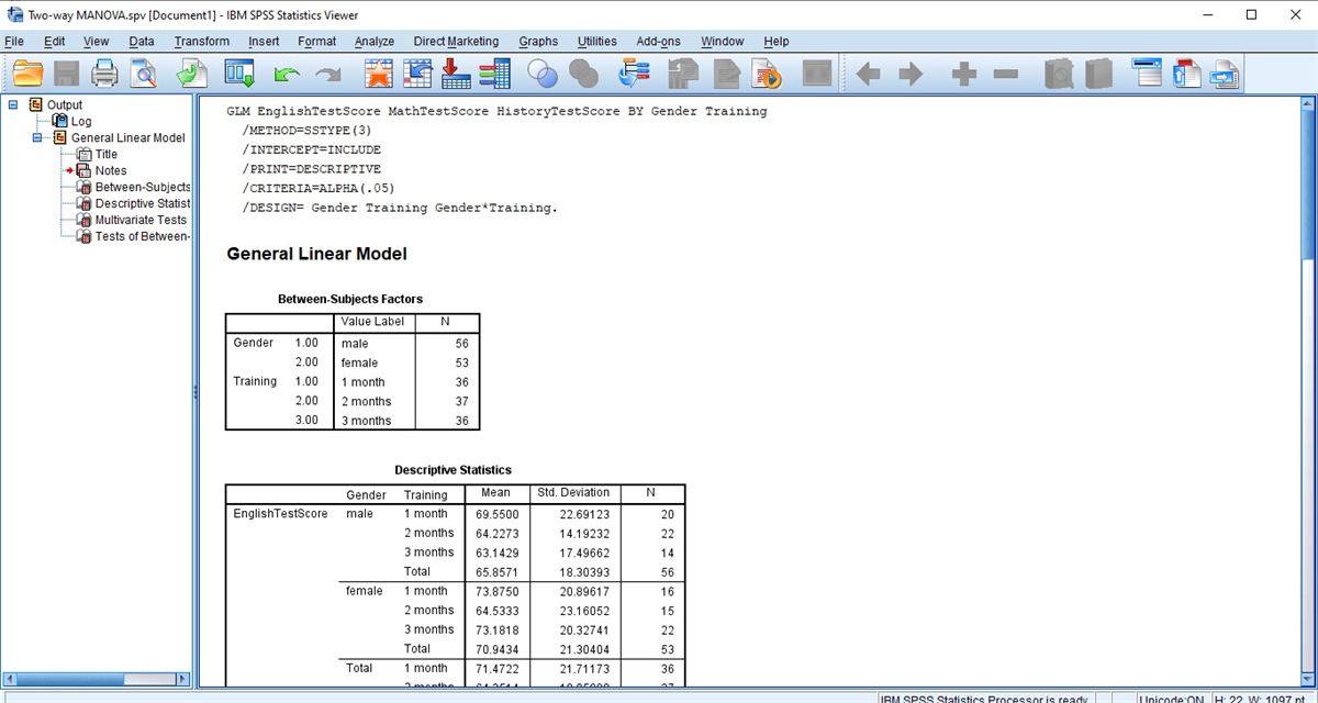
Open the Multivariate Dialog
Choose Analyze, then General Linear Model, then Multivariate. The Data Editor in the screenshot holds EnglishTestScore, MathTestScore and HistoryTestScore beside Gender and Training.
Check: Three outcomes tested across two between-groups factors belong in Multivariate. A factor measured on the same people several times needs Repeated Measures, listed in the same submenu.
Put Gender and Training in Fixed Factor(s)
Move the three test scores into Dependent Variables and both Gender and Training into Fixed Factor(s). The Model button keeps its defaults, and the syntax log later confirms Type III sums of squares and the full design.
Watch: The order of Gender and Training in Fixed Factor(s) changes no test result under Type III sums of squares. It only sets which factor forms the outer rows of Descriptive Statistics.
Keep Descriptive Statistics in Options
In Options, only Descriptive statistics is ticked and the significance level stays .05. Display Means for is empty, then select Continue and OK.
Tip: With this setting the output has no Box’s Test, Levene’s test, partial eta squared or marginal means. Homogeneity tests adds Box’s Test and Levene’s test, and Estimates of effect size adds partial eta squared.
Check the Syntax Log and Cell Sizes
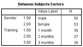
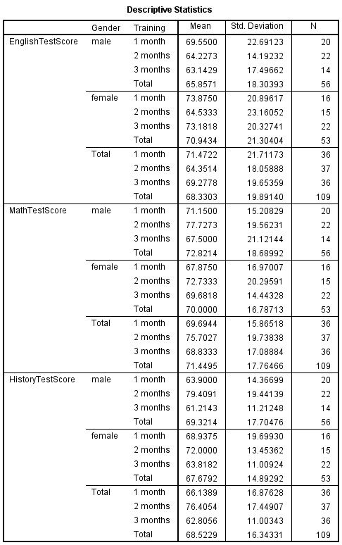
The Viewer opens with the GLM command (SSTYPE(3), PRINT=DESCRIPTIVE, DESIGN= Gender Training Gender*Training), then Between-Subjects Factors and a Descriptive Statistics table that lists each score’s mean, Std. Deviation and N cell by cell.
Watch: Between-Subjects Factors gives only the margins, 56 and 53 by gender and 36, 37 and 36 by month. The six cell counts appear in the N column of Descriptive Statistics, the smallest being 14 male participants at 3 months.
Read the Multivariate Tests Table
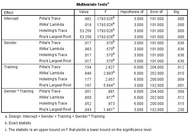
Four blocks appear: Intercept, Gender, Training and Gender * Training, each with Pillai’s Trace, Wilks’ Lambda, Hotelling’s Trace and Roy’s Largest Root. Start with Gender * Training, then the two main effects.
Tip: Error df differ by row: 101 for Gender, 202 for Wilks on Training, 204 for Pillai and 200 for Hotelling. Quote each F with the df printed on its own row.
Read the Tests of Between-Subjects Effects
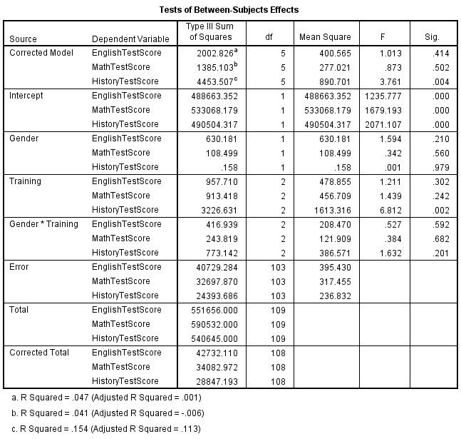
Each score has rows for Corrected Model, Intercept, Gender, Training, Gender * Training, Error, Total and Corrected Total. The effect rows use df 1, 2 and 2, with an error df of 103 for each score.
Watch: Three levels of Training mean a significant F does not say which months differ. This table holds no pairwise comparisons, and the video does not run the Post Hoc button.
READING THE OUTPUT
Reading Four Statistics for Each Effect and Score
Each row of the table names one value in the SPSS output, gives its figure in the video example and says how to read it for your own data.
| Output value | In the example | How to read it |
|---|---|---|
| N | Gender 56 and 53; Training 36, 37 and 36; total 109 | Cases per level. Cells hold 14 to 22 cases, and the error df of 103 is 109 minus 6 cells |
| Mean and Std. Deviation | History, male: 63.90 (14.37), 79.41 (19.44), 61.21 (11.21) for 1, 2 and 3 months | Cell means in test points. The six History SDs run from 11.01 to 19.70 |
| Gender * Training, Wilks’ Lambda | .950, F 0.877 (df 6 and 202), .512 | Read first. Pillai’s p of .509 and Hotelling’s .515 agree with it, and Roy’s row carries footnote c |
| Gender, Wilks’ Lambda | .983, F 0.570 (df 3 and 101), .636 | One df, so all four statistics are identical |
| Training, four statistics | Wilks .848, p .010; Pillai .154, .012; Hotelling .177, .009; Roy .167, .001 | Wilks and Pillai agree at about .01. The F tests differ in df and exactness, and footnote c applies to Roy’s row |
| Training row by score | English 1.211 (.302), Math 1.439 (.242), History 6.812 (.002), df 2 and 103 | Unadjusted univariate tests. Only History falls below .05 |
| Gender and interaction rows by score | Gender .210, .560, .979; interaction .592, .682, .201 | Sig. for English, Math and History in order, all well above .05 |
| R Squared (footnotes) | English .047, Math .041, History .154 (adjusted .001, -.006, .113) | Variance in each score linked to all five model df together, not to one effect |
COMMON MISTAKES
Slips With Roy's Root, Corrected Model and the Interaction
Some mistakes start in the data setup, others in the SPSS dialogs, the output or the write-up. Six of them follow, each with a short note on avoiding it.
Training Placed in Covariate(s) Coded 1, 2 and 3, Training can land in Covariate(s). It then becomes one slope with 3 multivariate df, and the default model drops the Gender by Training term. Wilks' Hypothesis df of 6 for Training confirms the factor.
Roy's p Quoted as the Result Roy's Largest Root gives Sig. .001 for Training, yet footnote c says its F is an upper bound, so that p is a lower bound. Wilks' lambda gives .010 and Pillai's trace .012, which are the safer figures to quote.
Corrected Model Taken as an Effect For History the Corrected Model row (F = 3.761, Sig. .004) tests all five model df at once. It is not the Training effect, whose row reads F = 6.812, Sig. .002, and it should not be quoted in its place.
A Large Interaction p Read as No Interaction A p of .512 gives no evidence of an interaction, yet the Gender gap could still differ between training lengths. Six cells of 14 to 22 cases leave room for sizable differences between gaps.
Training Wording That Implies Cause Nothing in the video says months of training were assigned at random. Without that, History scores differed by training length is the claim the data support, and training raised History scores goes further.
Total Rows Weighted by Cell Size In Descriptive Statistics the Training totals are weighted by cell size, for example 20 male and 16 female cases at 1 month. The Type III test compares means that treat both genders evenly, so the totals are a guide only.
If you have already run this test, Independent Statistical Review has an OnlineSPSS statistician check the interaction, then the statistic, against your output.
SOURCES
Sources and Further Reading
The sources below support statements made on this page, and the line under each entry says what to read it for.
Olson, C. L. (1974). Comparative robustness of six tests in multivariate analysis of variance. Journal of the American Statistical Association, 69(348), 894-908. DOI: 10.1080/01621459.1974.10480224
Read this for why Pillai's trace is preferred when assumptions are doubtful.
Lakens, D. (2013). Calculating and reporting effect sizes to facilitate cumulative science: A practical primer for t-tests and ANOVAs. Frontiers in Psychology, 4, Article 863. DOI: 10.3389/fpsyg.2013.00863
Read this for the definition and use of partial eta squared.
FREQUENTLY ASKED QUESTIONS
Menus, Partial Eta Squared and Month Comparisons in the Example
From the SPSS menus on your screen to the final write-up, the questions here follow this analysis, taking in the method and the video example.
Why does the Multivariate dialog look different in my SPSS?
The video was recorded in an older release of IBM SPSS Statistics. In the release 23 manual the Display list runs from Descriptive statistics to General estimable function, as it does here, and the significance level on that screen also sets the confidence level of the intervals.
Where is partial eta squared for Training on History?
Estimates of effect size is unticked in Options, so none is printed. From the table, 3226.631 / (3226.631 + 24393.686) gives .12 for History (Lakens, 2013), and the multivariate value for Training from Wilks’ lambda is about .08. Both were computed here, not read from SPSS.
Which training lengths differ on History?
The video stops at the F row. The Total means for History are 66.14 (1 month), 76.41 (2 months) and 62.81 (3 months), but pairs need the Post Hoc button or Compare main effects with an adjustment. Of the three Training rows only History, p = .002, clears a Bonferroni level of .05 divided by 3, or .0167.
How are Wilks' lambdas of .950 and .848 written up in APA 7?
Interaction first, then the main effects. A two-way MANOVA with English, Math and History as outcomes found no statistically significant Gender by Training interaction, Wilks’ lambda = .950, F(6, 202) = 0.88, p = .512, or Gender effect, Wilks’ lambda = .983, F(3, 101) = 0.57, p = .636, but a statistically significant Training effect, Wilks’ lambda = .848, F(6, 202) = 2.89, p = .010.
NEXT STEP
Need a Two-Factor, Multi-Outcome Design
Run or Checked?
OnlineSPSS is a statistical consultancy for researchers. Share your design and dataset, and a statistically trained Research Coordinator reviews it. The scope and one fixed project fee are confirmed before work begins.
No Commitment Required
Strictly Confidential
Fixed Project Fee
In-House PhD-Level Statisticians
Same-Day Response
Serving Researchers Since 2014