
Normality Tests in SPSS
Video Walkthrough With Shapiro-Wilk and K-S Tests
This normality tests in SPSS video asks whether age and height in 32 workers depart detectably from normality, using Explore. The page adds what each test can and cannot show, how to read the Q-Q plots and what form Age's departure takes.
WATCH THE VIDEO
Normality Tests in SPSS, Start to Finish
Decide what has to be approximately normal before any test is run: for most methods it is the outcome within each group, or the residuals, not the variable as a whole. Read Shapiro-Wilk as the main test, since it has better power than Kolmogorov-Smirnov even after the Lilliefors correction, and read it beside the Q-Q plot (Ghasemi & Zahediasl, 2012). In this example Age shows a detectable departure, and Height shows none that 32 cases can detect.
IN SHORT
What the Video Shows in Brief
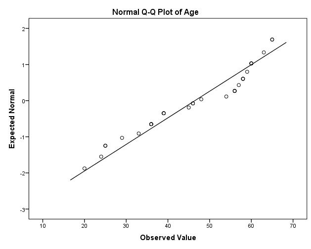
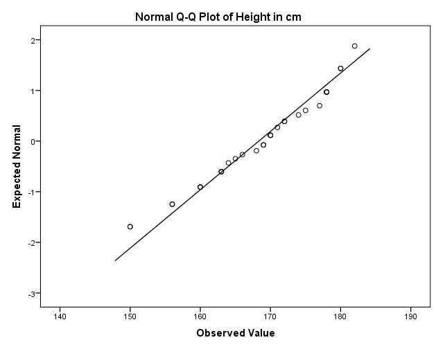
In this normality tests in SPSS video, Age and Height of 32 workers are checked in Explore with the Shapiro-Wilk and Kolmogorov-Smirnov tests and Q-Q plots. The path is Analyze, Descriptive Statistics, Explore, with Normality plots with tests ticked under Plots. Age shows a detectable departure from normality (Shapiro-Wilk W(32) = .917, p = .018), while Height shows none that 32 cases can detect (W(32) = .959, p = .256).
BEFORE YOU RUN
What Shapiro-Wilk and Q-Q Plots Need Before Explore
The four points below concern your study design and your data. Settle each one first, then run this normality check in SPSS.
Which Quantity Is Checked What must be near normal depends on the method: the outcome within each group for a t-test, the residuals for regression, the difference scores for a paired design. The video tests whole variables, as an illustration.
Sample Size Cuts Both Ways In small samples these tests have little power, so a non-significant result is weak evidence. In large samples they flag trivial departures (Ghasemi & Zahediasl, 2012), so the size of the departure matters more.
The Test Beside the Plot A significant test says a departure is detectable. The Q-Q plot, boxplot, skewness and kurtosis show its form and size, and a judgment about the method rests on these, not on the p-value alone.
Action Fixed in Advance Decide what a departure would change: a transformation, a robust method or a rank-based test that answers a different question. A plan made before the check keeps the choice from following the p-value.
STEP BY STEP
Running Explore With Normality Plots
Follow the numbered steps below through IBM SPSS, with screenshots as you go: each step gives the menu path, the settings to pick and a check or tip.
Numbered by step, the slides hold the SPSS screen one step at a time. Your release may label a few items differently, since the video was recorded in an older one.
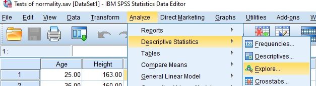
Open the Explore Dialog
Choose Analyze, then Descriptive Statistics, then Explore. The dialog opens with an empty Dependent List, Factor List and Label Cases by box, and the tests are requested later under Plots.
Check: Explore is the procedure that prints the Tests of Normality table. Frequencies and Descriptives can print skewness and kurtosis, but they print no normality test.
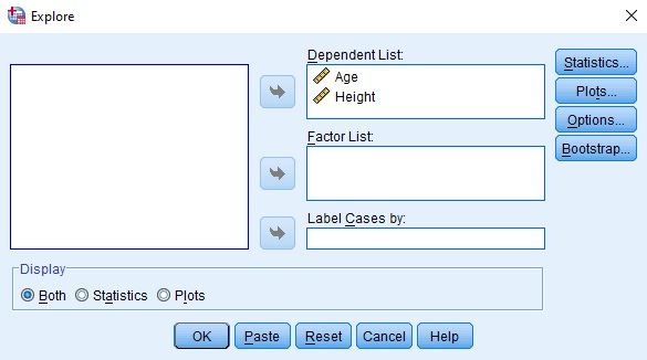
Move the Variables to the Dependent List
Move Age and Height into the Dependent List box with the arrow button, and keep Display on Both so that tables and plots are printed. The Factor List stays empty, so each variable is tested across all 32 cases.
Watch: An ID variable in Label Cases by makes the boxplot name each outlying case by its ID and not by its row number, which is easier to trace back to the data.
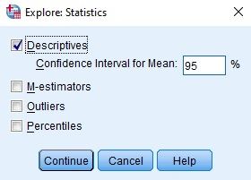
Ask for the Descriptives
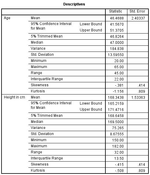
Select Statistics, keep Descriptives ticked with the confidence interval for the mean at 95, then select Continue. This prints the mean, median, skewness and kurtosis that the plots are read against.
Tip: M-estimators, Outliers and Percentiles are optional in the same dialog. Outliers lists the five highest and lowest values, which is useful when a boxplot shows extreme points.
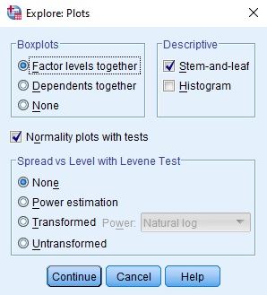
Ask for Normality Plots With Tests
Select Plots, keep Boxplots on Factor levels together, keep Stem-and-leaf ticked, tick Normality plots with tests, then select Continue and OK. The Histogram box is left unticked in the video.
Tip: Ticking Histogram as well adds a picture of the overall shape, which many readers grasp faster than a Q-Q plot, at the cost of one more chart per variable.
Check the Case Processing Summary
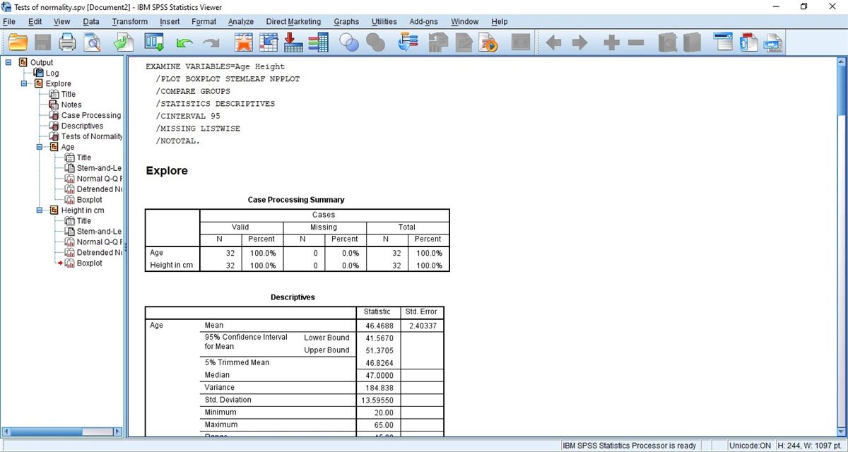
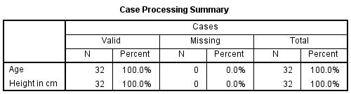
The Viewer shows the EXAMINE command, the Case Processing Summary, the Descriptives and the Tests of Normality, then the plots for each variable. Check the N in the Case Processing Summary before reading a test.
Check: Here N is 32 for Age and for Height with 0 missing, so both tests and both plots rest on the same 32 cases and the Age and Height rows of the table can be compared directly.
Read the Tests and the Q-Q Plots
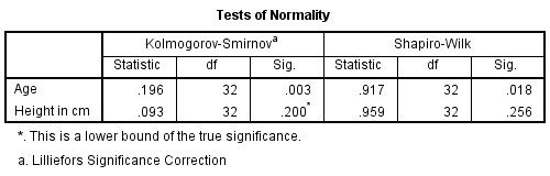
Read the Tests of Normality table, with Kolmogorov-Smirnov and Shapiro-Wilk side by side, then open each Normal Q-Q Plot. Judge the pattern of the points against the line, not one point alone.
Watch: The Viewer also lists a Detrended Normal Q-Q Plot for each variable. It plots each point’s distance from the line, so a curve there shows the same pattern at a larger scale.
READING THE OUTPUT
Reading the Tests of Normality and Q-Q Plots
Each value below comes from the SPSS output. Its row shows the figure in the video example, then how to interpret it when the data are your own.
| Output value | In the example | How to read it |
|---|---|---|
| N and Percent (Case Processing Summary) | 32 valid and 0 missing, for Age and Height | The cases that entered the tests, to be read before any test statistic |
| Mean and 95% CI | Age 46.4688 (41.5670 to 51.3705), Height 168.3438 (165.2159 to 171.4716) | The location of each variable, as context for the plots. It is not a normality statistic |
| Median and 5% Trimmed Mean | Age 47.0000 and 46.8264, Height 169.5000 and 168.6458 | Close to the mean here, which suggests little asymmetry in either variable |
| Skewness and Kurtosis | Age -.381 and -1.156, Height -.415 and -.508 | The direction of the tails and their weight, each with its standard error (.414 and .809) |
| K-S Statistic, df and Sig. | Age .196, 32 and .003, Height .093, 32 and .200* | Lilliefors-corrected. The .200* means p of .200 or more, not exactly .200 |
| Shapiro-Wilk Statistic, df and Sig. | Age .917, 32 and .018, Height .959, 32 and .256 | W near 1 means close to normal. A small p flags a detectable departure, and a large p shows none that N can detect |
| Normal Q-Q Plot | Age: runs of points on both sides of the line; Height: points close to the line | The form and size of the gap, not a verdict. Tied values draw darker circles |
COMMON MISTAKES
Explore Slips From the Factor List to the Q-Q Plot
Six mistakes with this normality check are set out below. Each comes from the data setup, dialogs, output or write-up, with a short note on avoiding it.
Treating Every Departure as Skew Age's skewness is only -.381, while its kurtosis of -1.156 points to a flat, light-tailed shape. Name the form of the departure, since light tails trouble a test of means far less than a long tail does.
No Factor Entered for Group Comparisons With the Factor List empty, the tests describe the pooled variable. A comparison of groups needs the grouping variable there, so that each group gets its own test and Q-Q plot.
Normality Plots Option Left Unticked Without Normality plots with tests under Plots, Explore prints descriptives and boxplots but no Tests of Normality table and no Q-Q plot. Tick it before OK and confirm the table in the Viewer.
Listwise Exclusion Across Variables Explore excludes cases listwise by default, so a case missing Height also leaves the Age test. Check the Case Processing Summary, and use the Options button when each variable should keep its own cases.
Over-Reading One Point on the Q-Q Plot The lowest Height value, 150 cm, sits furthest from the line while the rest follow it. Judge the pattern across the plot, and read a darker circle as several identical values on one spot.
Plot and Missing-Value Settings Not Saved The EXAMINE command above the tables shows NPPLOT, which requests the tests, and MISSING LISTWISE. Save it in a syntax file beside the .spv output, so both settings can be checked when the analysis is reviewed.
If you have already run these tests, Independent Statistical Review has an OnlineSPSS statistician check the test, the plots and the wording against your output.
SOURCES
Sources and Further Reading
A note under each reference says what to read it for, and every reference listed supports a statement on this page.
Ghasemi, A., & Zahediasl, S. (2012). Normality tests for statistical analysis: A guide for non-statisticians. International Journal of Endocrinology and Metabolism, 10(2), 486-489. DOI: 10.5812/ijem.3505
Read this for how the normality tests compare and why sample size matters.
Lilliefors, H. W. (1967). On the Kolmogorov-Smirnov test for normality with mean and variance unknown. Journal of the American Statistical Association, 62(318), 399-402. DOI: 10.1080/01621459.1967.10482916
Read this for why K-S needs a correction when the mean and SD are estimated.
FREQUENTLY ASKED QUESTIONS
Menus, the Starred p and Test Disagreement in the Example
Each question below concerns this analysis in SPSS: why a screen may differ from the video, a point of method, a figure in the example or the write-up.
Why does the Explore dialog look different in my SPSS?
The video was recorded in an older release of IBM SPSS Statistics. Release 29.0.1 redesigned the Statistics sub-dialog of Explore, with its own variable list and Missing and Bootstrapping buttons, and added a Percentiles dialog for quartiles or custom percentiles. Step 3 therefore looks different, while the Tests of Normality table is read as in the video.
Why does Height show .200* instead of an exact p-value?
The Kolmogorov-Smirnov row uses the Lilliefors significance correction, which is needed because the mean and SD are estimated from the data (Lilliefors, 1967). SPSS prints .200* when p is .200 or more, and the footnote calls it a lower bound of the true significance. Report p > .200 for that row.
Why do the two tests give different p-values for Age?
They measure departure in different ways, and one data set can put either p below the other: here Kolmogorov-Smirnov gives .003 and Shapiro-Wilk .018. Both are below .05, so both flag a detectable departure. Where they disagree, Shapiro-Wilk is the better-powered test (Ghasemi & Zahediasl, 2012).
How are W(32) = .917 for Age and .959 for Height written up?
With the test, its statistic, df and p for each variable, and the shape evidence. Shapiro-Wilk: Age W(32) = .917, p = .018; Height W(32) = .959, p = .256. Age shows evidence of a departure from normality (skewness -0.38, kurtosis -1.16). The Height result is not proof that its distribution is normal.
NEXT STEP
Need Normality Tests and Q-Q Plots
Run or Checked?
OnlineSPSS is a statistical consultancy for researchers. Share your design and dataset, and a statistically trained Research Coordinator reviews it. The scope and one fixed project fee are confirmed before work begins.
No Commitment Required
Strictly Confidential
Fixed Project Fee
In-House PhD-Level Statisticians
Same-Day Response
Serving Researchers Since 2014