
Kruskal-Wallis Test in SPSS
Video Walkthrough of a Worked Happiness Example
This Kruskal-Wallis test in SPSS video asks whether happiness ratings from 1 to 5 differ across five marital status groups. The page adds why the Chi-Square row is H, what mean ranks near 14.5 show and how to word a p-value of .956 for 28 people.
WATCH THE VIDEO
Kruskal-Wallis Test in SPSS, Start to Finish
Plan the comparisons before the Kruskal-Wallis test is run. H answers one question, whether the rank distributions of all the groups are alike, and cannot say which groups differ. Pairwise follow-ups based on rank sums are adjusted for the number of comparisons (Dunn, 1964), so the pairs worth testing are named beforehand. Here H is not significant, so the finding is stated as no evidence of a difference, not as equal happiness.
IN SHORT
What the Video Shows in Brief
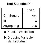
In this Kruskal-Wallis test in SPSS video, happiness ratings from 1 to 5 are compared across five marital status groups of 28 people: single (5), married (6), divorced (7), widowed (5) and separated (5). The path is Analyze, Nonparametric Tests, Legacy Dialogs, K Independent Samples, with Define Range 1 to 5. SPSS prints Chi-Square = .661, df = 4 and Asymp. Sig. = .956: not statistically significant.
BEFORE YOU RUN
What Five Groups of Ratings Need Before Ranking
Here are four points to settle about your study design and your data, each one ahead of running the Kruskal-Wallis test in SPSS.
Unrelated People Each person gives one happiness rating and belongs to one marital status group. Two spouses from one married couple, or the same person rated twice, break that independence and need a model for linked ratings.
Five Ordered Levels Ratings from 1 to 5 are ordinal, and the test uses only their order. That, and not a normality check, is what justifies a rank test for this scale.
Married Versus Single Shapes Look at the distribution of ratings within each group. A statement about group medians needs similar shapes, and here they differ: the married group has two 1s and three 5s, while the single group stays between 1 and 4.
Ties and Approximation A five-point rating produces many ties, and SPSS adjusts H for them. The p-value rests on a chi-square approximation to H (Kruskal & Wallis, 1952), so with groups of five to seven an exact p-value is worth requesting where licensed.
STEP BY STEP
Running K Independent Samples With Define Range
Screens are pictured as they appear in IBM SPSS, and each numbered step below sets out the menu path, the settings to select and one check or tip.
Each slide shows the SPSS screen for one step and carries its step number. The video was recorded in an older release, so labels on your screen may differ slightly.
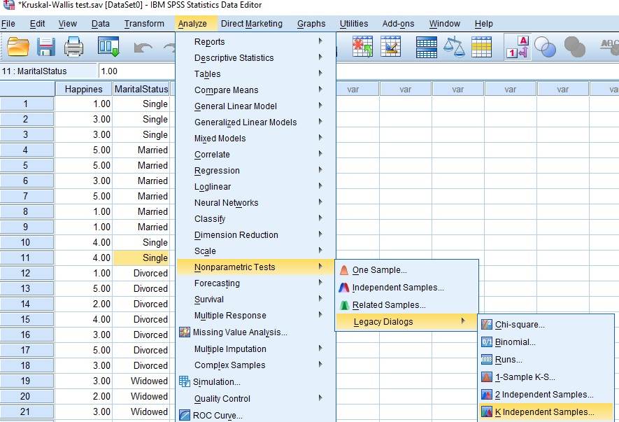
Open the K Independent Samples Dialog
Go to Analyze, Nonparametric Tests, Legacy Dialogs and pick K Independent Samples. The K stands for the number of groups, which is five in this example.
Check: The entry just above is 2 Independent Samples, which compares only two groups. Running it pair by pair for five groups gives ten unadjusted tests in place of one.
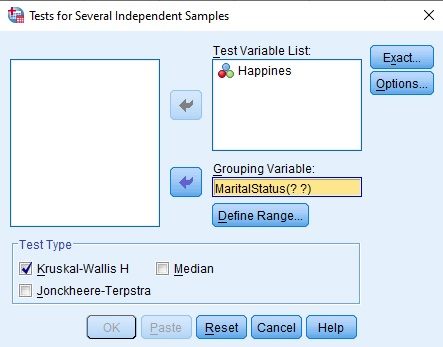
Move Happines and MaritalStatus Into Place
Happines, the rating, goes into Test Variable List, and MaritalStatus into Grouping Variable, which shows MaritalStatus(? ?) until Define Range is used. Of the three test types, only Kruskal-Wallis H is ticked; Median and Jonckheere-Terpstra stay off.
Watch: The icon beside Happines marks it as nominal in the data file, although the ratings are ordinal. The test still runs, but set the level to Ordinal in Variable View so the file describes the variable correctly.
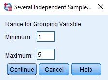
Set Minimum 1 and Maximum 5 in Define Range
Define Range wants the lowest and highest group codes: type 1 as Minimum and 5 as Maximum, then Continue. The five groups listed later in Ranks, from Single to the one the output prints as Separate, all fall inside.
Check: Every case with a code from the minimum to the maximum is included, so a code for missing marital status that falls inside the range would form a group of its own.
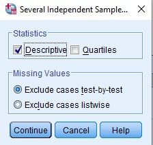
Tick Descriptive Only Under Options
Open Options, tick Descriptive only, accept the default Missing Values setting, Exclude cases test-by-test, and press Continue, then OK. The video leaves Quartiles unticked.
Tip: Leaving Quartiles off is fine for the test; it changes only the Descriptive Statistics table, never H or its p-value.
Count the Five Groups in the Viewer
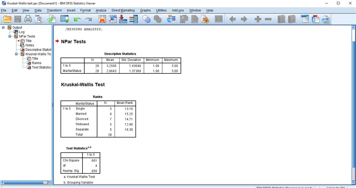
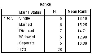
Three tables appear in the Viewer. Before H, read the N column of Ranks: 5 single, 6 married, 7 divorced, 5 widowed and 5 separated people, 28 in all.
Check: Compare the Ranks total with N in Descriptive Statistics, both 28 here. Descriptives counts every rating, while Ranks keeps only cases with a group code from 1 to 5, so a gap shows people lost to the grouping variable.
Read the Descriptive Statistics Table
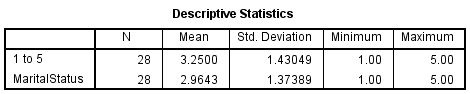
The rating row shows 28 valid values with a mean of 3.25 and an SD of 1.43, from a lowest rating of 1 to a highest of 5.
Check: The output names the outcome by its variable label, here 1 to 5, not by its name. A label such as Happiness rating (1 to 5) keeps the tables readable without the data file.
Read Mean Ranks and the Chi-Square Row
In Ranks, each marital status group has an N and a mean rank, without rank sums. Test Statistics then prints Chi-Square, df and Asymp. Sig., and footnote b names MaritalStatus.
Tip: The mean ranks, 12.90 to 16.30, sit close to 14.50, the mean rank of all 28 ratings. That closeness is what an H near zero looks like.
READING THE OUTPUT
Reading H Where SPSS Prints Chi-Square
Each value below comes from the SPSS output. Its row shows the figure in the video example, then how to interpret it when the data are your own.
| Output value | In the example | How to read it |
|---|---|---|
| N, Mean, Std. Deviation | 28, 3.2500, 1.43049 | Whole-sample summary on the 1 to 5 scale, which the test itself does not use. Round to 3.25 and 1.43 if quoted |
| Minimum and Maximum | 1 and 5 | Both ends of the rating scale occur in the data |
| N in Ranks | Single 5, Married 6, Divorced 7, Widowed 5, Separate 5 | People per group, with the fifth group labeled as the output prints it. They add up to 28 |
| Mean Rank | 13.10, 15.25, 14.71, 12.90, 16.30 | Each group’s average place among the 28 ratings, with tied ratings sharing an average place. Ratings tied at 5 share places 21 to 28, so each gets 24.5 |
| Chi-Square | .661 | The Kruskal-Wallis H statistic, adjusted for ties |
| df | 4 | The number of groups minus one, here five groups |
| Asymp. Sig. | .956 | The p-value from the chi-square approximation to H with 4 df. It does not measure how far apart the groups are |
| Footnotes a and b | Kruskal Wallis Test; Grouping Variable: MaritalStatus | Name the test and the grouping variable. Check both against the analysis plan before quoting the result |
COMMON MISTAKES
Slips With the Chi-Square Label and Group Codes
The six slips below happen while setting up the data, working in the SPSS dialogs, reading the output or writing up, and each has a note on prevention.
Causal Wording for Existing Groups Marital status is recorded, not assigned, so the test compares ratings across existing groups. Write that happiness ratings were compared across groups, never that marital status affects happiness.
Chi-Square Reported as Another Test The row labeled Chi-Square is the Kruskal-Wallis H statistic, and it has nothing to do with the chi-square test on a crosstab. Label it H with its df, as H(4) = 0.66, and name the test in the sentence.
A Trend Test on Unordered Groups Jonckheere-Terpstra in the same dialog tests an ordered trend across the group codes. Marital status codes 1 to 5 have no order, so a trend result would depend on how the categories happened to be numbered.
Ordinal Ratings Summarized by the Mean A mean of 3.25 treats the gaps between rating levels as equal, which an ordinal scale does not promise. Give the number of people at each level, so that the pattern within each group is visible.
Groups Merged After the Result With groups of five, merging categories to enlarge them is tempting. Merge only by a rule written before the test, since a regrouping chosen after seeing the mean ranks changes what the p-value means.
Define Range 1 to 5 Not Saved The range sits in the command, MaritalStatus(1 5), and not in any table. Paste the syntax and keep it with the output and a dated copy of the data, so a later recode cannot change which five groups were compared.
If you have already run this test, Independent Statistical Review has an OnlineSPSS statistician check the H label, the pairs and the wording against your output.
SOURCES
Sources and Further Reading
A note under each reference says what to read it for, and every reference listed supports a statement on this page.
Kruskal, W. H., & Wallis, W. A. (1952). Use of ranks in one-criterion variance analysis. Journal of the American Statistical Association, 47(260), 583-621. DOI: 10.1080/01621459.1952.10483441
Read this for the H statistic and its chi-square approximation.
Dunn, O. J. (1964). Multiple comparisons using rank sums. Technometrics, 6(3), 241-252. DOI: 10.1080/00401706.1964.10490181
Read this for multiple comparisons that are based on rank sums.
FREQUENTLY ASKED QUESTIONS
Menus, Follow-Ups and Effect Size in the Example
Questions on the Kruskal-Wallis test follow, from a screen that looks different in SPSS through the method and the video example to wording the result.
Why does the Tests for Several Independent Samples dialog look different in my SPSS?
The video was recorded in an older release of IBM SPSS Statistics. In release 30, Tests for Several Independent Samples still sits under Analyze, Nonparametric Tests, Legacy Dialogs, and its Define Range button works as in the video. IBM’s page for that release asks for integer values in Define Range.
How do I get pairwise comparisons after a Kruskal-Wallis test?
The legacy dialog in the video prints the omnibus test only. The Independent Samples item under Nonparametric Tests offers pairwise comparisons, with significance values that SPSS adjusts for all ten pairs of the five groups. Here H is not significant, so the example calls for none.
What effect size belongs beside H(4) = 0.66?
The legacy output stops at Chi-Square, df and Asymp. Sig., with no effect size. Epsilon squared, H divided by N minus 1, is .66 / 27, about .02 here and close to zero. With five to seven people per group that estimate is imprecise, so give it with the group sizes rather than alone.
How is a non-significant H(4) = 0.66 for 28 people worded?
With H, its df, the sample size and the p-value. A Kruskal-Wallis test did not reach statistical significance, H(4) = 0.66, p = .956, N = 28, with mean ranks from 12.90 (widowed) to 16.30 (separated) and an epsilon squared of about .02, in groups of five to seven people each.
NEXT STEP
Need Five-Group Ratings
Run or Checked?
OnlineSPSS is a statistical consultancy for researchers. Share your design and dataset, and a statistically trained Research Coordinator reviews it. The scope and one fixed project fee are confirmed before work begins.
No Commitment Required
Strictly Confidential
Fixed Project Fee
In-House PhD-Level Statisticians
Same-Day Response
Serving Researchers Since 2014